

GEOMETALLURGY
SOFTWARE
User Manual v2.7

© 2019-2026 Transmin Metallurgical Consultants
All rights reserved. No parts of this work may be reproduced in any form or by any means - graphic, electronic, or mechanical, including photocopying, recording, taping, or information storage and retrieval systems - without the written permission of the publisher.
Products that are referred to in this document may be either trademarks and/or registered trademarks of the respective owners. The publisher and the author make no claim to these trademarks .
While every precaution has been taken in the preparation of this document, the publisher and the author assume no responsibility for errors or omissions, or for damages resulting from the use of information contained in this document or from the use of programs and source code that may accompany it. In no events are the publisher and the author liable for any loss of profit or any other commercial damage caused or alleged to have been caused directly or indirectly by this document.
Table of Contents
Introduction
Overview
Cancha is an integrated solution for geometallurgical sample selection, result interpretation and reporting.
Cancha is used by geologists, miners, metallurgists and geometallurgists to accurately, efficiently and transparently project metallurgical performance for mineral resources.
Its specialized geostatistical functions help ensure that metallurgical samples accurately represent the broader ore deposit, reducing uncertainty in test results. This improves confidence in metallurgical testwork results and reduces financial risk to mining companies.
The analysis and interpretation module uses advanced data science, analytics and machine learning to propose prediction algorithms for each parameter of interest. These parameters typically include recovery, product quality, operating cost and throughput rates, however Cancha has the flexibility to provide robust predictions for any measured parameter.
Thanks to the integrated reporting module, the documentation and presentation of geometallurgical models is fully automated, facilitating knowledge transfer, audits and reviews.
Cancha is an indispensable tool for geometallurgical interpretation for large, medium and small mines, base metals, precious metals, industrial minerals, light metals, PGM’s, coal and shale oil and more.
Cancha raises the bar for reporting standards in metallurgical performance projections. It was developed to aid the geometallurgists, but it is valued by investors for bringing confidence and transparency to mine economic models.
Functions include:
Drill logs visualization and statistical analysis
Block model visualization and statistical analysis
Metallurgical sample selection, visualization and representivity audit
Metallurgical testwork analysis and interpretation
Geometallurgical prediction algorithm generation
Model quality and confidence metrics
Automated documentation and reporting
Name
Cancha is a Quechua word, used in Peru for “field” (both one’s field of professional expertise and a football field). It’s also used for popcorn.
Cancha is a Peruvian word, for a Peruvian geomet software, for the world.
Exclusions
There are many things that Cancha is not:
Customizable. Many software packages are difficult to learn because people spend a lot of time choosing colors, fonts and layouts. We have opted for the approach where formatting decisions are already made, allowing the user to focus on the content. We do acknowledge that there are some circumstances that our choices are not perfect.
Multi language. We made it in English. In the distant future we may consider offering other languages, but for the time being, it is only in English.
Rigid. Cancha does not enforce specific units of measurement or geological classifications. Whether you use feet, meters, or fathoms is up to you. Cancha does not know if a metallurgical feature is a hardness test or a recovery. The user has to take care.
Apple, Linux compatible. We have only developed it for 64-bit Windows systems.
GIS. Cancha is not built to hold all versions of all geospatial data for a mine. It is a tool for analysing the latest version of drill holes, block models and geometallurgical testwork.
Resource, reserves mine plan, mass balance tool. In order to keep the workflow simple, there are many features that will not be added to Cancha. There are great software packages available for geological modelling, mine planning and process design. Cancha should not be used for any of these things.
Opensource. Our algorithms are not transparent. The results are. Cancha will suggest geometallurgical models, sample selection and domains. Supporting statistics show why these are theoretically good choices, but we do not claim that these are correct nor optimal. The user has to use knowledge of the deposit geology and metallurgy to validate the suggestions from Cancha.
Colors
There are just a few different color schemes in Cancha. The idea is to help the users spend their time on analysing data and not on making it pretty.
 Numerical feature colors
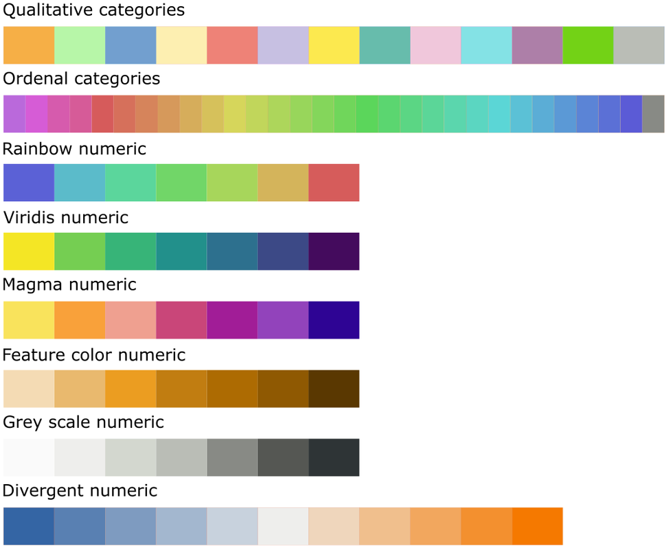
Numerical features are arbitrarily assigned a base color from one of 29 colors.
This color, and the tones for it from light to dark are what are used by default to show data in 3D, Logs and Analysis.
In the 3D Controls window you can change the color scheme used for drilling, block model or samples to other schemes, according to your personal taste and the work at hand.
The Rainbow scheme was added under duress and we are a hair away from taking it out again.
When looking at the data it is useful to have an even and continuous progression in color contrast and intensity to avoid misunderstandings.
The developer of the Viridis color scheme gave an excellent talk on how this color map works, and why it is so much better than the rainbow alternative that is more common, but less useful. Yellow is used for low values, as it is close to the white background.
Dark purple is used for high values, as it has the most contrast with a white background.
In a world where we are used to seeing warm colors as high and cool colors as low, it takes some practice to get used to Viridis, but it is worth the effort.
 Categorical feature colors
Categorical features are represented by either nominal or ordinal colors.
Nominal features are assigned one of 12 colors. They are designed to have high contrast between them, both in hue and value, but in general, these colors are arbitrary.
Ordinal features are assigned colors in the rainbow sequence, in order to show a progression between them.
In both cases, the grey color on the end is used to cover minor or ignored bins.
 Colors for analysis and reports
Where distance from the average is interesting, a diverging color scheme can be helpful.
For example, reviewing recovery in 3D, it might be interesting to highlight the different extreme high and extreme low recovery samples, essentially ignoring the average recoveries.
The divergent scheme applies:
Low values are blue
Average values are grey
High values are orange
Fonts and text
All labels, tables, captions and other texts in Cancha use the OpenSans font. Changing text size, color and style are not possible as we are trying to keep the interface clean and encourage the user to think about the science rather than the aesthetics.
Nomenclature
Feature - Any data column that can be used in the analysis.
Objective - The final input to mine planning. Tonnage, for example is simulated from ore particle size and hardness, for example.
Target - The feature that will be used to describe the variability in the block model. The Bond ball mill work index, for example.
Numerical - A feature that comprises useful numeric values, such as zinc grades between 0 and 100%.
Ranges - A numeric range that is used to bin or categorize numerical data. For example, RQD of 0-25%, 25-50% and 50-100%
Categorical - A feature that comprises of qualitative data, such as lithology that may be binned as skarn or breccia
Principal - the list of key drivers from the features that most affect the metallurgical performance
Sample - A metallurgical sample is a single interval of drill core from a single drill hole.
Composite - A metallurgical composites are blends of different samples.
Focus case - the resource that you want the geomet samples and predictions to represent.
Sample frame - the subset of the drilling that the samples will be taken from.
Domain - A domain is a bin or category of a categorical feature that can be used to usefully describe a portion of the orebody.
Spatial domain - used to describe a geographical area of the orebody, such as splitting the orebody into “Central”, “Northern” and “Eastern” zones.
Period domains - if you already have a mine plan, then domains can be made by year or phase, for example
Geological domain - This could describe any geological event that can be modelled. For example, porphyry lithology, supergene mineralization, or vein structure
Grade domain - Blocks can be binned according to their grade, either pay metals or other interesting grades. For example, high grade gold, or low grade arsenic
Areas
The main toolbar in Cancha guides you through the project workflow, from left to right.

Start by setting up the project data:
 Info. Set up basic information that will be used in report headers.
 Data. Import, delete or export data.
 Table. View the data in tables.
 Features. Set up your feature colors, groups, names, and derive new features.
 Filters. These are global features that affect all of the other areas.
Next view and analyse the data:
 3D. Safer than skydiving over the project.
 Logs. View drilling data and select samples using strip logs.
Analysis. Graphs and statistics.
 Pivot. Create and export tables that summarize cross referenced data.
Finally generate your models and reports:
 Samples. Metallurgical sample tools and summaries.
 Targets. Generate models, compare and select your favorite.
Working With Cancha Files
Cancha joins together data from many different sources into a single database for review, analysis and reporting.
The project is stored in a .gmt (geomet) file. This file can be transferred between computers, including all of the data, settings and analysis.
⚠️ | Important: Avoid Cloud-Synchronized Folders |
Create a new project
When you open Cancha, you are presented with this screen:
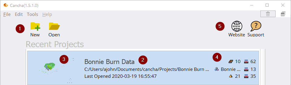
File operations:
 Create a new project. Start from zero.
 Open an existing project. Open an existing .gmt file and continue working.
Recent projects are listed
The “favorite view” is used for a thumbnail
Here we see some summary information about the project:
 The number of drill holes in the project
 The name of the block model
 The number of samples in the project
The number of features in each area
While only one project can be open at a time per instance of Cancha, more than one instance of Cancha can be running on a single computer, so if multiple projects need to be open, simply open another instance of Cancha.
Saving gmt files
 With every user action, Cancha updates the data set and feature parameters. Therefore, the gmt file is automatically saved after each operation and there is no undo functionality.
If you want to keep historical records, it is recommended that you archive backup copies of gmt files periodically.
Project Information
Take the time to add the project information when you start a new project.
This information will be used by Cancha when it comes to naming samples and designing reports.
Add company, client and project names and logos once, and they will be added to the reports automatically.
The history tab shows you all of the actions that have been completed in the gmt file.
Data Manager
The Data Manager area is where the following data types can be imported:
Table data
Drilling data
Block models
Metallurgical sample data
Origin
Characteristics
Test parameters
Test results
3D shells
Open surfaces
Closed volumes
The following options are available in the Data Manager view:
 Add data
 Delete data
 Export Cancha project
Obtaining data
Advice on how to obtain data for a Cancha model is provided here (links to Cancha Data Guide document).
Import data
Follow these steps to import data:
Click on the
Add File icon. Select the file(s) to be imported. Multiple files, tables and shells can be imported at once.Specify the file type to be used
Data Type and Columns window appears. Identify the name of the columns in which Hole ID, From, To and others specifications are located if required. Cancha makes a guess, but it can be mistaken, so be sure to check.
The original names are what appears in the data file that is imported
The new names can be edited. Cancha will change some names automatically, such as N, E, RL
Cancha guesses the feature type, if incorrect then change it between numerical, categorical or text. Change of attribute types by clicking the label. Categorical Data (geological attributes), Numerical data (chemical assays for example), Text (notes, observations).
You can choose to ignore any feature and this feature wont be imported.
You can choose to trim a feature. After selecting this option, Cancha will prompt you to set filter criteria during import. Only data rows that meet your criteria will be imported into the project.
This area shows examples of the data to be imported. It is not a faithful preview of the actual table, rather it finds random rows from the file to use as example data.
The Skip button is used to skip the import of the information displayed
Once the configuration of the next table is finished, press Next to go to the next table
Important: All coordinates must use the same projection/datum system as your drilling data. Mixed coordinate systems will cause spatial alignment errors.
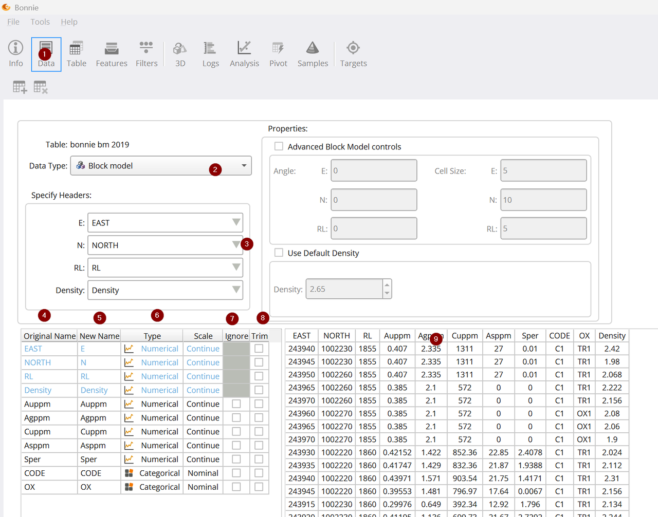
Table data
Cancha can import table data from the following file types:
Comma delimited CSV files (best for block models and drilling)
Excel Spreadsheet XLS & XLSX files (best for metallurgy)
File format DM files (very slow)
Template files
Cancha can import your existing data in the original Excel or csv (comma delimited) text files, so long as you have:
the right header columns
Just one header row.
All unique header field names.
No merged cells.
Cancha can create a metallurgical data template Excel file for importing data that is already set up for best practices. Find it in the menu “Tools/Templates”
Drilling data
Drilling data is typically a series of tables, each with a different set of data for the same holes.
These tables typically include some of the following:
Collars (obligatory)
Survey
Assays
Lithology
Alteration
Mineralization
Geotechnical
Block model data
The block model is an arrangement of regularized blocks distributed in space. The complete set of volumes represents the global geometry of a given resource.
Block model files must contain as a minimum the following three fields:
Easting
Northing
RL, Elevation
Other common block model fields are not required by Cancha, but can be imported if desired.
Examples include:
Block numbers, i, k, l
Block dimensions
Relative local location, x, y, z. Only world locations are useful as they must coincide with the drilling and shell coordinates.
All other fields are likely useful for geometallurgy and should be imported as features, for example:
Metal grades
Geological domains
Mining phases or periods
Mining domains
Resource category
Net smelter return value
Block dilution information
Geotechnical values
In situ rock density
In some cases, the block model may be rotated about an axis. In this case, there should be additional information accompanying the block model, that explains:
Which axis was rotated, x, y, or z
What was the angle of rotation
Video Tutorial |
|

Another special case is that of sub-cell block models. These block models are not regularized. There are no standards for sub-cell block models, but usually there is a maximum cell size that relates back to a regularized block model size. Cancha cannot display sub-cell models, but it can import the files, and by forcing a single block size, one is able to work with the data, albeit with errors for blocks that were divided.
🛑 When sub-cell models are imported in this way, the visualization and look-ups will be simplified, and distorted. However, the table that is imported is the complete original table, so any graphs or statistics will be correct.
Shells
Shells can be imported in dxf format. These files can generally be in one of two types:
Open surface, like a sheet of paper
Closed volume, like a balloon
In both cases, they can be visualized in the 3D view, and used to create categorical features for drill holes and block models.
The accuracy of the importation process for these files into Cancha depends on the quality of the original file that is imported. If there are sparse nodes then the imported shell may be of low accuracy, as Cancha will interpolate a surface between the nodes.
Note that the dxf format is a general format and the data contained can vary. Some popular mine planning software has the ability to export dxf files of pits that are not surfaces or volumes, rather they are a series of lines. Cancha cannot interpret a dxf file if it does not contain the 3D model as a surface or a volume. |
If the name of the shell is red in the 3D Controls list, then it is far from the rest of the data.
Typically this means that the 3D file has been coded with relative coordinates rather than local coordinates. Cancha cannot fix that. The software that produced the shell should be configured to export the shell using world coordinates.
Metallurgy
Metallurgical information should be imported in separate tables, the same way that drilling information is. This will facilitate navigation and analysis of the information in Cancha. In some geometallurgical studies, over 1000 features can be developed for each sample. Keeping the information well organized is important to being able to work quickly and accurately.
Video Tutorial |
|
Metallurgical information should be imported in separate tables as follows:
 Origin. The sample origin table should have the following fields:
Sample ID
Drill hole
From
To
Phase
There should only be one sample origin entry for each sample in Cancha.
 Characteristics. This group of information describes the characteristics of the sample as it was extracted from the drill core tray, such as:
Head grades
Geological parameters such as lithology, alteration
Geotechnical parameters such as rock quality, density, particle size or moisture content
Mineralogical information such as mineral assemblage, texture or associations
Each of these can and should be imported as a separate table.
Characteristics tables must have a Sample ID and Phase fields.
 Test parameters. This data is test specific. The conditions of the tests, such as particle size, reagent regimes, time, temperature or flowsheet are imported here.
Test parameter tables must have a Sample ID and Phase fields.
Each type of test should be imported as a separate table, for example, comminution, flotation and leaching test parameters should be in separate tables.
 Results. Test results are imported here, and may later be declared as targets for geometallurgical analysis. Typical results may include recoveries, reagent consumption or concentrate grades.
Results tables must have a Sample ID and Phase fields.
Each type of test should be imported as a separate table, for example, comminution, flotation and leaching test parameters should be in separate tables.
Composite. Existing metallurgical composites can be imported.
Composite tables must have Phase ID, Sample ID and a column for each composite. The header should be the name of each composite, and the data should include numbers, such as mass of each sample used in each composite.
Tables
Since most of the data that is used in Cancha is tables, these tables can be viewed by the user. Typically this view is only used for error investigation, as Pivot Tables, graphs, and other advanced reports are usually more useful than reviewing the tabular data.
Clicking on a feature in the Feature List will bring up the table and column that it comes from.
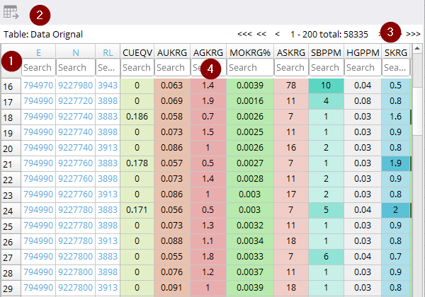
The blue text columns indicate the table header columns for the table
The table can be exported as a csv file. This can be useful when derived features have been created that can be used in other software.
Scrolling through massive data tables is hard to do, and actually not very useful. Basic navigation controls are supplied, but it is expected that search, filters or pivot tables would be used by most users.
Numerical and logical text searches can be used to find the rows of interest. It behaves like a filter for the feature, but does not affect the other data structures in Cancha.
Categorical features can be searched by typing part or all of the search term. Logical boolean operators or wildcards do not work. The search is not case sensitive. Any part of the string can be used.
For example, “A” will find “MAG” or “ARC”
Numerical features can be searched for values or ranges.
For example, >0.2, or <=1.5
Features
In the world of geometallurgy there are no standards for terms, and so it is common for data to be described as data, fields, parameters, x-data, columns, criterion, inputs and more.
When developing Cancha, we decided to adopt the nomenclature used by many in data science. The term “feature” is used to describe a table column, or data field that is available for analysis.
All of the data that is imported into Cancha, including geological, mining and metallurgical information, is considered to be a set of features.
Objectives
Cancha is used for geometallurgical analysis in order to determine values for Objectives that will be used by mine planners. Users will be surprised to discover that Cancha does not actually develop these objectives for the user. The fundamental idea of geometallurgy is that low quality, abundant variability data is used in conjunction with high quality, sparse, calibration data, in order to project objectives over a resource. The objectives are therefore not related to the geometallurgical analysis itself, rather the objectives are simulated from the targets.
Objective = function (Target)
Examples:
FinalRecoveryCu = RougherRecoveryCu - 3%
Tonnage = function (Bond Ball Work Index)
Targets
In Cancha, the Target is the field from the metallurgical results table that will be modeled. This model will be used to predict the target value in each cell of the block model using geological features.
Features
Data that can be modeled spatially and populated in the block model. These typically include geological logging, chemical analysis and geotechnical logging data.
Samples used for geometallurgical tests need to be classified by these same features, using the sample basis.
Feature engineering is used for target modeling. In this step, features are classified by degree of predominance in the chosen target.
Each section represents the multivariate regression on a group of samples. Sections vary depending on the number of samples with complete data sets.
The Feature List is on the left of the screen for most Areas.
| There are three ways that the Feature List can be shown: |
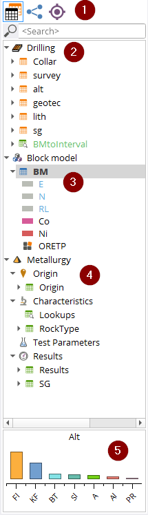
The features sub-types are: principal, calculated, interpolated and ignored.
 Features
 Ratio
Ratio
 Derived feature
Interpolated features
 Shell to drill hole
 Shell to block model
 Samples Distances
 Mapping Shells
 Links
Links
Ignored. The user should decide if it is better to:
Ignore features during the importation process, and they will not appear in Cancha
Ignore features that are already imported. This can be valid, and improves transparency if they are ignored explicitly.
 Legend Editor
Either right-click on a feature in the Feature List, or choose a feature and click on the Features Area to bring up the Legend Editor.
This is where numerical and categorical data is whipped into shape prior to analysis.
Numerical Legends
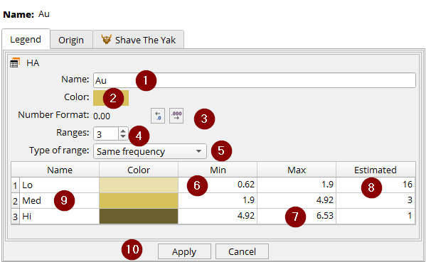
Rename the feature
Choose the feature base color
Specify the number of decimals for this feature
Specify the number of ranges (Lo, Med, High = 3 ranges in this case)
Choose the distribution type:
Same frequency, creates ranges with approximately equal numbers of data points
Same width, creates mathematically equal intervals
Cluster, uses k-means algorithm to find natural data groupings
Custom, allows manual range definition
The minimum value, cannot be edited
The maximum value, cannot be edited
This only estimates the population in each range. If you want an exact number, use the statistical tools in the Analysis area.
Rename the ranges as required.
Hit apply, or else all of the changes will be lost.
Categorical Legends
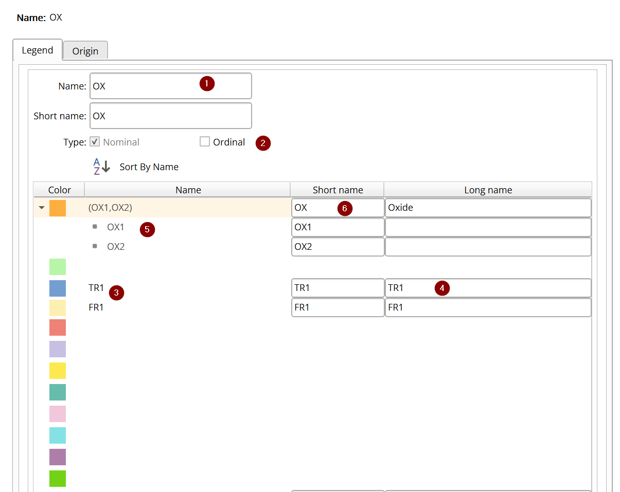
Rename the feature
Choose:
Nominal for unrelated bins
Ordinal for bins that have a progression, such as Mining Phases, for example
There are a maximum of 12 bins. The top 12 most popular categories are used by default, the rest are grouped in “Others”
Rename each bin as required
Group categories into a single bin using the mouse to drag them around. Also use the mouse to select the order and color of each bin
Short names are automatically generated, but can be edited, they should be 6 or fewer characters.
Hit apply, or else all of the changes will be lost.
Note that the colors cannot be changed.
Derived features
Derived features are new numeric features that are calculated from existing features.
The formula syntax comes from the muParser Fast Math Library that is used behind the scenes.
Built-in functions
Use these mathematical functions to create new features from existing data. For example, use log() to normalize highly skewed grade data, or sqrt() to calculate geometric means.
The following table gives an overview of the functions supported.
Name | Explanation |
sin | sine function |
cos | cosine function |
tan | tangents function |
asin | arcus sine function |
acos | arcus cosine function |
atan | arcus tangens function |
sinh | hyperbolic sine function |
cosh | hyperbolic cosine |
tanh | hyperbolic tangents function |
asinh | hyperbolic arcus sine function |
acosh | hyperbolic arcus tangents function |
atanh | hyperbolic arcur tangents function |
log2 | logarithm to the base 2 |
log10 | logarithm to the base 10 |
log | logarithm to base e (2.71828...) |
ln | logarithm to base e (2.71828...) |
exp | e raised to the power of x |
sqrt | square root of a value |
sign | sign function -1 if x<0; 1 if x>0 |
rint | round to nearest integer |
abs | absolute value |
min | min of all arguments |
max | max of all arguments |
sum | sum of all arguments |
avg | mean value of all arguments |
Built-in binary operators
The following table lists the binary operators that can be used.
Operator | Description | Priority |
&& | logical and | 1 |
|| | logical or | 2 |
<= | less or equal | 4 |
>= | greater or equal | 4 |
!= | not equal | 4 |
== | equal | 4 |
> | greater than | 4 |
< | less than | 4 |
+ | addition | 5 |
- | subtraction | 5 |
* | multiplication | 6 |
/ | division | 6 |
^ | raise x to the power of y | 7 |
Ternary Operators
“if then else” functions can be achieved by using next syntax:
Condition ? Value if true : Value if false
Example for assigning 92% Cu Recovery for CuT grade greater than 0.15%, or 50+280*CuT for lower grades.
(CuT>0.15) ? 92 : 50+280*CuT
Look-up features
Values from the drill hole intervals are composited into the Samples interval. The averages are based on length, varying density is not considered.
 Ratio
Ratio
The ratios are reasons that provide units of measurement and comparison, through which it is possible to analyze the data obtained.
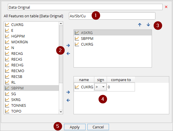
Name the ratio
Add from two to six numerical features to the ratio list
Choose the order that you want to see them
Filter the ratio, so it only shows up under certain criteria. For example, sequential copper ratios can be meaningless for very low grade total copper values, so filter for values over the cut off grade.
Apply to create the ratio
Once created, it can be used as a feature in Logs.
 Linked features
Right now this does not do much in Cancha. In order to implement transfer of metallurgical information back to the block model and drill holes, it will be necessary to link the corresponding features. For example, if a copper recovery model requires the copper head grade, based on metallurgical test head assays, then in order to implement copper recovery in the block model, we will have to identify the copper head grade feature in the block model.
This will be important in the future, for now it is just a placeholder.
 Block model to drill hole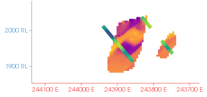
The block model to drill hole interpolator passes the categorical and numerical values from the block model to the drill holes automatically. The data appears as a new  Lookup table in the Drilling data section of the Feature List.
Shell to block model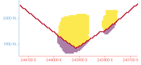
The shell to block model interpolator populates the block model with categorical “in” or “out” ordinal values, from 3D shells.
The data appears as a new feature in the Block model section of the Feature List.
A second feature is also created that gives the distance for each block to the shell.
 Block model to Shell
In the 3D view, click on the block model to shell button to generate a shell using the block model geometry that is visible at the time. Any filters, or ranges that are hidden will not be included in the mesh.
Shell to drill hole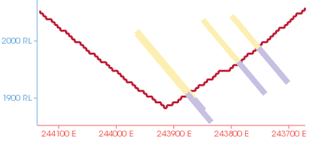
The shell to drill hole interpolator populates a new Drilling table with categorical “in” or “out” ordinal values, from 3D shells. If shells come from an open surface, Cancha arbitrarily choses “A” and “B” values for this derived feature. These can be renamed as “in” and “out” in the Legend editor, for example.
The data appears as a new Lookup table in the Drilling data section of the Feature List.
 Domain classifier
The domain classifier uses an ordered algorithm to create new features in Drilling, Block model, or Metallurgy tables.
Video Tutorial |
|
A series of logical expressions is used to sort the population into two or more domains.
All of the conditions in a label are “and”. There is no “or” functionality.
Only features from the same table can be used. If features from other tables are required, then they should be interpolated using other feature tools before using the Domain classifier.
Both Categorical and Numerical features can be used.
Categorical features that are to be included should be selected in the checklist
Numerical features are classified by equality formulae (<,>,=, etc)
Not all blocks should be “true” in a classifier. The final category should be the remainder, though you do not have to call it the remainder, the name can be edited.
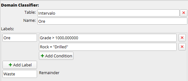
The new feature will appear as a new regular categorical feature in the table that was used to derive it.
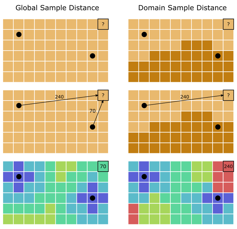
Sample distance feature
This tool generates a new feature in the block model table. It gives the minimum distance to a metallurgical sample, either in the global set, or in a domain system.
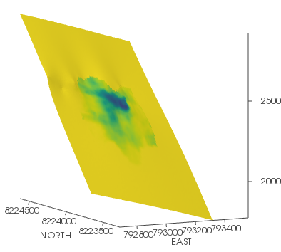
 Shell data mapping
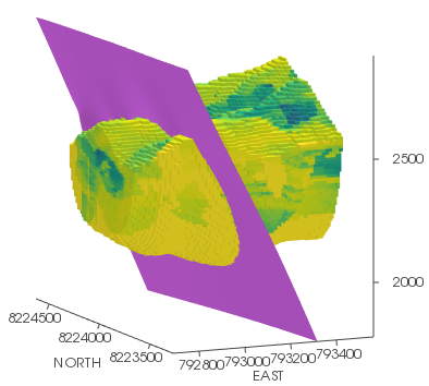
You can bake a block model feature to the shell using the shell data mapping tool, found in the Features Area.
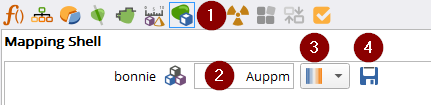
Choose the shell mapping tool
Drag the feature that will be mapped from the block model section of the Feature List
For numeric features, choose which color scheme will be used
Hit the save icon to bake the block model feature to the shell
 Shave the Yak
If the numerical data columns that are imported contain text, or other non-numerical characters, then Cancha will crash!
Shaving the Yak is an important and onerous task for the geometallurgist.
Here is a checklist of steps to get your data in shape for analysis:
Integrate data. Single tables for drill collars, or sample origin can facilitate the work flow.
Group similar features. Navigating features is easier when they are grouped together in tables.
For example, keep head assays and mineralogy in separate tables for metallurgical samples.Consolidate data. Often there may be multiple columns in a table that have to be interpreted together as a single feature. Consolidate these columns before importing them.
For example, zinc assays on drilling may be found as part of an ICP column, but where the assays were high (>1%), a second column shows the results of a zinc determination by AAS. Therefore, it is recommended to create a third column with the best values from each assay, and only use that as the zinc assay feature.
Another common example is in geological rock type logs. There may be dozens of rock types identified, but a pragmatic review could reduce them to 5 or 6 groups, which would be more useful as potential domain systems.Treat null data. Depending on how the data was produced, there may be different terms for null (empty) data values. Common examples include “Null”, “-”, “N/A”, “-999”, or simply no value at all. Cancha only works if null values are given as either empty or “-”.
Remove data leakage. Data leakage is where the target value is present in a separate feature, but should not be used as a predictor.
For example, a Bond work index file may have grams per revolution and BWi in separate columns. Model generation will identify this feature as an excellent predictor of hardness, but it should not be used as it comes from the metallurgical testing and not the knowledge of the geological deposit.Treat erroneous data. If data is erroneous, do not use it for analysis.
For example, if metallurgical tests failed due to poor mass balances, incorrect conditions, or spoiled samples, then do not use this data for analysis.Rectify duplicates. Have the same features or samples been incorporated twice?
For example, if duplicate tests were run for quality assurance purposes, then they should be reviewed and removed or treated before use in analysis.Review extremes. Most geometallurgical numerical data is greater than zero. Outliers can confuse the clustering and learning algorithms.
For example, if 99.99% of the data is below 2%, and one value is 30% Cu, then that one value adds more noise than value, and should be removed or reduced.Homologize scale. Have ppm, ppb, and % been mixed in the same feature? Metric vs short tonnes? Make sure that all values in a feature are on the same scale.
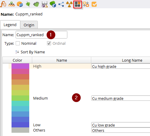
 New category from ranges
This tool generates a classification from a Numerical Feature into a categorical feature, for example we can generate a distribution from Cu Low grade, Cu Medium grade and Cu High grade.
Put the numerical feature in this area, it will renamed automatically into a Categorical name
In this area edit the names of each category
 Change data type
With this tool a numerical feature can be transformed into a categorical feature and also a categorical feature can be transformed into a numerical feature
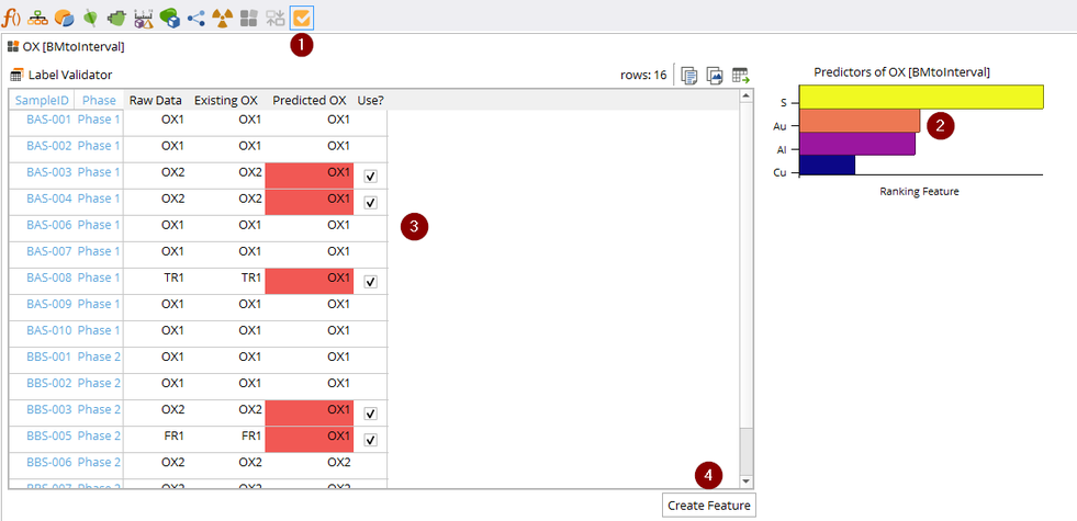
 Label Validator
This tool is used to validate categorical features based on numerical variables.
Numerical values are used as predictors
This area shows the confirmation or denial of the categorical label
Finally press Create feature to create a new validated feature
Clustering Drilling Data
In the realm of geochemical data analysis, clustering is a pivotal technique for identifying patterns and trends within drilling assays. Our toolkit introduces two robust clustering methods: Segmenting and Smoothing. Each offers a unique approach to streamline data interpretation and enhance sample selection.
Segment Data
Simplifies exploration drill data by identifying and highlighting lengths of assays with similar geochemical values. This contrasts with surrounding intervals, making the identification of significant geochemical trends more efficient.
Right click on the feature you want to cluster in the Feature List, and select “Segment”
In a few seconds, a new feature will appear below the feature, with the postscript “smooth”.
Before it can be used, you will need to reconsolidate the drilling data using the orange button at the extreme top right of the screen.
Smooth Data
Sorts geochemical assay data into high, medium, and low categories, then creates clusters of continuous intervals within these ranges, applying the average grade to each interval.
Right click on the feature you want to cluster in the Feature List, and select “Smooth”
In a few seconds, a new feature will appear below the feature, with the postscript “smooth”.
Before it can be used, you will need to reconsolidate the drilling data using the orange button at the extreme top right of the screen.
Mineral Calculator
Reference: Bill Whiten (2007): CALCULATION OF MINERAL COMPOSITION FROM CHEMICAL ASSAYS, Mineral Processing and Extractive Metallurgy Review: An International Journal, 29:2, 83-97
The mineral composition calculator integrated enables users to deduce mineral composition from chemical assays. It utilizes the methodology described in the paper by Bill Whiten (2007), "Calculation of Mineral Composition from Chemical Assays," published in the Mineral Processing and Extractive Metallurgy Review.
Adding Minerals
Initiate Mineral Addition: To add minerals to the list, click the green cross symbol.
Select Minerals: Type the name of the desired mineral. A list of minerals will appear based on the input. Select the appropriate mineral from this list to add it to your calculation.
Assigning Chemical Assays
Consistent Source: Ensure that all chemical assays used are from the same source and units of measure. The source can be drilling, block model, or metallurgy data, but these should not be mixed.
Drag and Drop Assays: For each element required, drag the corresponding chemical assay from the feature list into the input box provided for that element.
Recommendations and Precautions
Completeness of Assays: While it is possible to infer some element compositions, having a complete set of assays for the elements in the list is preferable.
Understanding the Methodology: Users are strongly encouraged to read and understand the paper by Whiten (2007) before using the calculator. This understanding is crucial to avoid errors in calculation and interpretation of results.
Finally, hit the Apply button, and the minerals will be added as new features to the same table as the assays came from.
Filters
The Filter is the only tool in Cancha that affects the fundamental dataset that is used for calculations and analysis.
Other search boxes, and radio buttons in the viewing areas hide data, but do not exclude it from consideration.
The filters remove all data that corresponds to the exclusions. For example, if high iron drill intercepts are filtered out, then all of the other drill hole data that corresponds to high iron grades are also excluded. It is not just the iron grade feature that is removed, but the entire drill intercept where there is high iron.
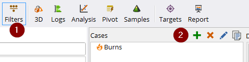
Click the Filter area
A case is a set of filters that focus the data in Cancha, for example “oxides”, or “Early years pit”. These operations are available for cases:
 New case
 Delete case
 Edit case
 Duplicate case
Numerical filters
A numerical filter is created by dragging a numerical features from the feature list to the filter case area.
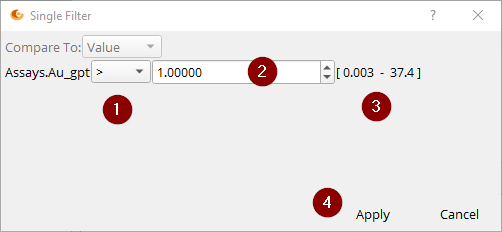
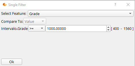
Choose the operator for the data that will stay in the analysis. In this case, drilling that is less than or equal to 1 g/t Au will be filtered out.
Set the value
This is the range of the values in the feature. Cancha will not allow you to filter outside the existing range to avoid errors.
Click Apply or Cancel to finish.
Categorical filters
For categorical data, it is a similar process.
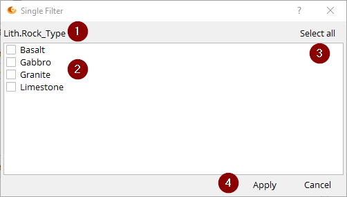
Drag a categorical feature from the feature list to the filter area. In this case we chose the Rock_Type feature in the Lith table.
Choose the categories that you want to keep.
Select all is also available.
Click Apply or Cancel to finish.
Managing Case Filters
One gmt file can be set up with several different case filters, allowing the user to switch back and forth between scenarios. For example life of mine, versus specific production periods.
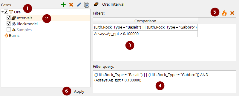
The cases can be activated and deactivated individually, as can the specific drilling, block model and metallurgy sample filters within each case.
Select an area, in this case Drilling Intervals, to see the filters associated with it on the right.
Individual filters can be added, or deleted here.
The SQL query is shown here for transparency, but is not editable.
Each filter can be burned into the gmt file, or deleted from the case.
Click Apply or else your changes will be lost.
Note: Filter processing time depends on dataset size and computer performance. Small projects: 1 minute. Large projects: 5-10 minutes. An alternative approach is to maintain separate .gmt files for different scenarios. This happens because when the data set changes, Cancha consolidates, cross-references, summarizes and otherwise re-calculates everything again from scratch. When the filters are removed, it has to do it all over again.
We recommend choosing carefully before using filters, and find something else to do. An alternative is that you could keep different copies of the project .gmt file on your computer, and have multiple instances of Cancha running. While one is running filters, you could be using the other instance to work on another aspect.
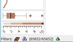
Do not forget when you have filters active! You may get in trouble if you prepare reports or publish models on partial data. Icons appear in the bottom left of the screen as a reminder that you have filters active. |
Burn Filters
Sometimes project data can include drilling from outside the area of interest, or a block model that goes from sea level to the moon. In these cases Cancha can be slow as it is processing a lot of redundant data.
The Filters area allows the user to hide redundant data, but the data is still there, and is being filtered for every operation, slowing down performance.
At the users discretion, it might be more convenient to burn the data that is not required.
This is done by:
First apply the filters as normal in the Filter area.
Check that the data that has been filtered is correct and that nothing extra has been excluded by mistake
In the Burns tab of the Filters area, choose to burn the filter for the drilling, block model or samples.
This will permanently and irreversibly remove that data from the Cancha .gmt file.
The burn is stored as a text for reference in the burns list.
⚠️ WARNING: Burning filters permanently and irreversibly removes data from your .gmt file. Ensure you have a backup before proceeding.
3D
All of the drilling, block model, shells, and metallurgical sample data in Cancha can be visualized in 3D together.
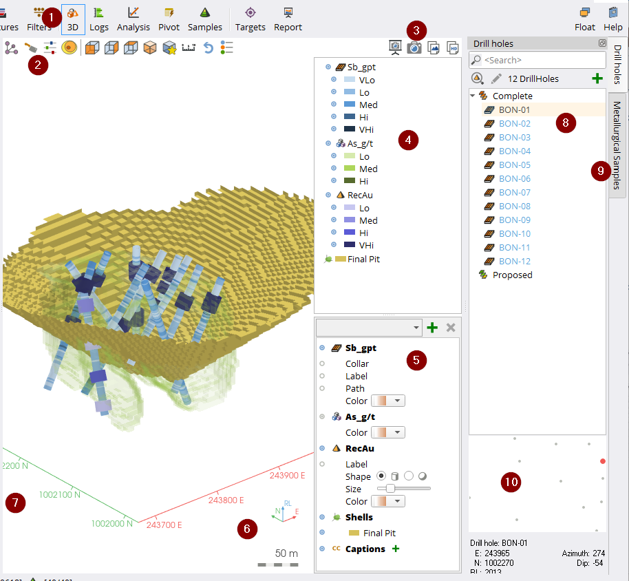
Select the 3D area
Tools for viewing the data in different ways in 3D
Tools for exporting reports and images
An interactive legend that can be used to show/hide data dynamically
Controls for choosing colors, labels and visibility of different data types
Indication of orientation and scale
Axis for N, E, and RL
The searchable and clickable drill hole list
The searchable and clickable metallurgical sample list
The clickable plan view of the drill collars.
3D Controls
Drilling Data
Collars - shows a blue marker at the collar
Labels - shows the drill hole name at the collar
Path - shows the drill hole string as a line
Color - choose the color scheme for numerical data
Block model
Color - choose the color scheme for numerical data
 Shells
Color- choose the color, or map a feature
Metallurgical samples
Labels - show the sample name
Shape - choose either a cylinder for the length of the intercept, or a sphere at the center of the intercept
Size - change the diameter of the sphere or cylinder
Color - choose the color scheme for numerical data
 Caption
Text captions can be added to the view. The text is anchored to a 3D point, then rotates so that it is always facing the camera.
The 3D controls toolbar has all of the elements that are currently in the viewport.
The user can turn on or off any of these elements as follows:
 Element view on
 Element in semi-transparent ghost view
 Element view off
Views
Saved Views
Video Tutorial |
|

Legend
The Legend tool in the 3D viewer will place a legend over the 3D viewport that will be captured by screenshots.
The legend can be dragged around with the mouse inside the viewport.
 Bounds
The bounds icon draws a bounding box around the input data extents, allows selecting and trimming giving limits to the deposit.
A bounding box is a three dimensional box that extends around the input data extents.
Note that changing the bounds does not filter the data in Analysis, it only changes the data that is viewed.
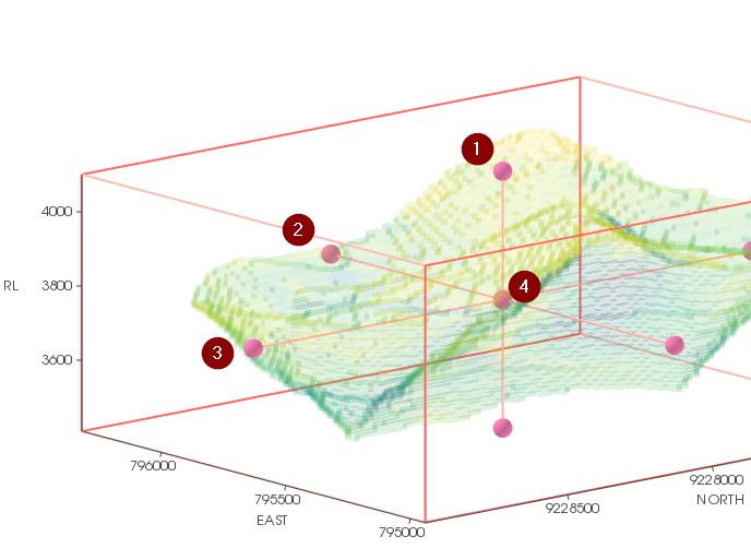
Adjust the upper limit
Adjust the western limit
Adjust the southerly limit
Move the entire bounds box laterally
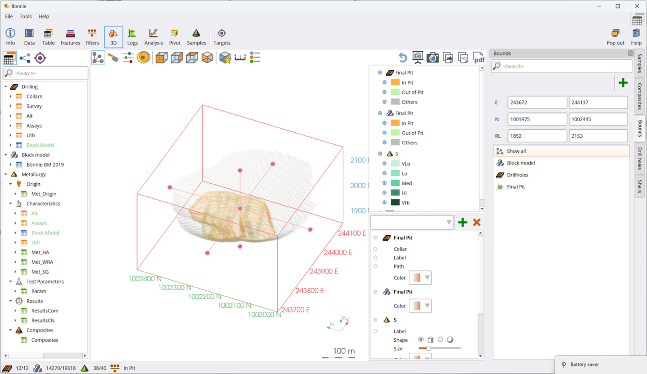
A window on the right hand side of the screen appears.
Maximum and minimum coordinates for each axis can be added manually.
The list of saved bounds is automatically populated with “Show all”, block model, drilling, and shell bounds. Additionally, users can set up custom bounds, and save them using the green cross button.
Once the bounds have been set up as required, click on the bounds button again to exit bounds mode.
 Section
The 3D section tool allows to visualize a slice of the deposit
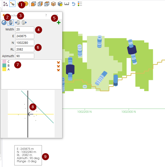
Select the section view from the 3D area toolbar
Switch back and forth between 3D and 2D
Step back and forth perpendicular to the section plane
The width is both the distance that is stepped, and the depth of drilling, and samples that are captured in the section.
Save the current active section in the list
Manually specify the center point of the section plane
A clickable and color coordinated list of saved sections
An interactive map in plan view of the saved sections
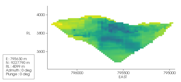
The section view shows the section coordinates
Video Tutorial |
|
Moving to the 2D section view, the camera automatically zooms onto the section plane to fill the viewport.
 Splitter
You can get a view of the three orthogonal planes through the block model data by clicking the splitter icon.
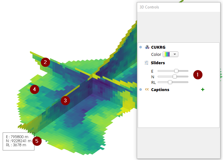
Move the three planes using the sliders in the 3D Controls toolbar.
The East plane
The North plane
The RL plane
The coordinates of the intersection between the three planes is shown
 Isosurface
The Isosurface tool removes all blocks in the block model with values lower than the value chosen. This tool only affects the block model view.
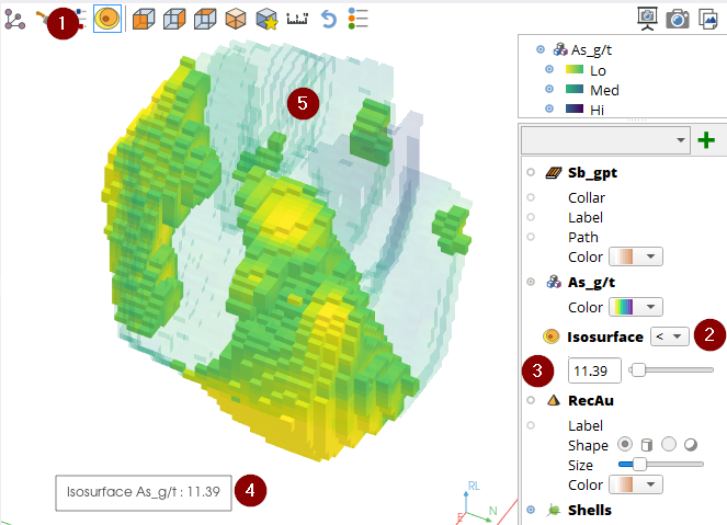
Activate isosurface mode.
Choose if you want to look at high or low values.
Enter the value of interest, or use the slider
The value used is shown
The blocks with higher values are ghosted
 Measurement
To measure a distance, click the mouse at the start and end positions. The distance measured is given in the plane parallel to the computer screen.
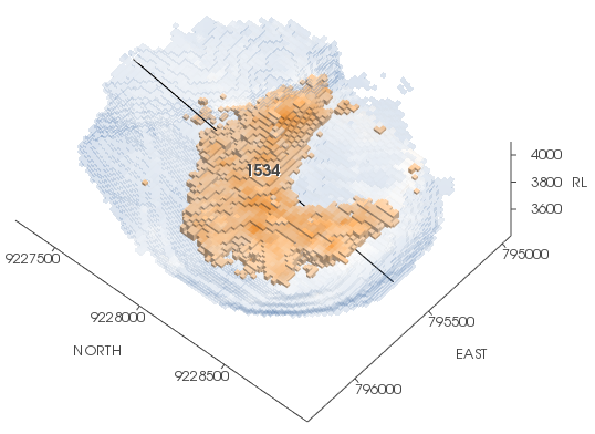
The following tools are available for different views in 3D:
Perspective:
 View looking North
 View looking West
 View looking down
 Isometric view from the south east
 Screenshots
 Captures multiple preset views with the current features to the project Report
 Copy current 3D scene to clipboard (ctrl+c shortcut too)
 Refresh
Update the viewport manually. It should update automatically, but we added this button just in case.
Logs
Logs is a tool to visualize drilling data. The user can view sample intervals, alteration zones, lithology, assays, etc.
The categorical data is colored and labelled according to the grouping in the Legend editor.
The numerical data takes the shape of vertical bars charts, and are colored according to the Legend color and intensity. Light colors for low values and dark colors for high values.
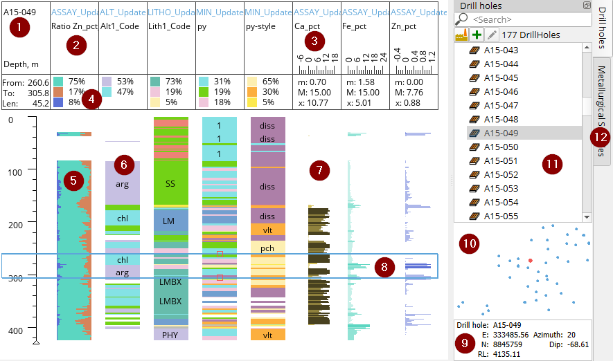
Drill hole name
Strip chart headers:
Ratio features are presented as stacked graphs
Categorical features are presented as color strips with labels
Numerical features are presented as vertical bar charts
Numerical features have fixed scales for all drill holes. The scale maximum is not the maximum value in the database, rather it is the 95th percentile value.
The summary bar gives summary data for the selected range (8):
Categorical data is given as the percentage of length in the selected interval, of each category. Only the top three are shown.
Numerical features show the minimum (m), maximum (M) and average (x) value for the selected interval.
Ratio features are colored according to the individual feature colors in the Legend editor.
Categorical features are colored according to the grouped colors in the Legend editor. Labels for categorical data are hidden if the intervals are too short. Zooming in will expand the view and labels will appear.
Numerical data is not labelled by default, but can be useful for metallurgical test results, for example. To add labels to numerical strip logs, right click the header and select “Show labels”. If the interval lengths are too short on the screen, the labels will not appear.
The user can select any intervals in different ways:
clicking and dragging the mouse over the log.
double-clicking any interval in any strip log to select that entire interval
Choosing a metallurgical sample from the list (12) to jump to that hole and sample.
The drill hole collar information is given.
A plan view mini-map of the drill collars is given, not to scale. Blue dots represent all of the holes, the selected hole is highlighted in red. Click on a blue dot to select that hole.
Drill holes can also be selected by clicking on them in the drill hole list. Holes that are given in blue text are holes that have metallurgical samples.
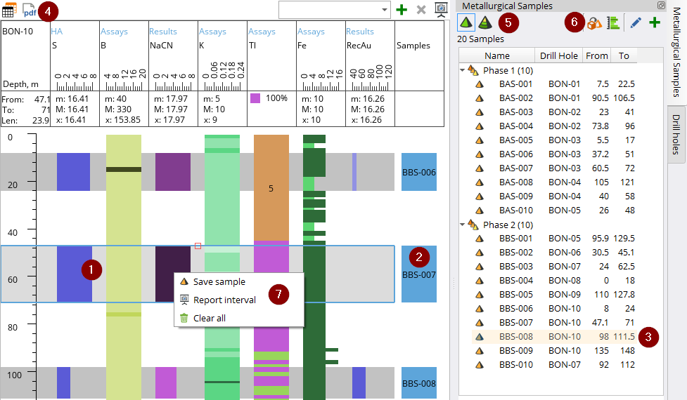
Existing samples can be quickly reviewed by reading across the grey band.
The name of the sample is given at the right side of the screen. The color of the sample name bar depends on the phase of the test sample.
Each metallurgical sample can be specified by the drill hole name, the From-To interval. Clicking on the sample will take you to that drill hole and interval.
All holes, the current hole or selected interval can be copied to the clipboard, sent to a report, or exported as a pdf file.
Do not forget that samples and composites are listed separately.
Change into 3D view to see the sample in reference to drill holes, blockmodel and shells
Right-click on a selected interval to save a sample, export a graphic, or clear a selection.
Interactions
To add a strip log, dragging the feature from the Feature List to the Log view.
Delete strip logs by double clicking on the header.
Zoom in and out in Logs by holding the Ctrl button on the keyboard and scrolling with the mouse wheel.
The default view has the entire length of the hole on the screen, regardless of the hole depth. If the user uses zoom to see more detail, the mouse scroll wheel can be used to scroll up and down.
There is no limit to the number of logs that can be added, but the typical screen can only show about 6 to 10 strip logs at once. If more are added, then they will be lost to the right of the screen.
Analysis
The Analysis section provides statistical tools and visualizations to explore relationships in your geometallurgical data, identify patterns, and support decision-making for sample selection and model development. These tools help you understand correlations between geological characteristics and metallurgical performance before proceeding to formal modeling in the Targets section.
Overview of Analysis Tools
The analysis tools are organized by the type of insight they provide:
Exploring Relationships Between Variables
Matrix Plot - Displays correlation matrices to quickly identify which features are related to each other. Use this to find unexpected relationships or confirm geological hypotheses across multiple variables simultaneously.
XY Scatter Plot - Examines detailed relationships between two specific variables, with options to color-code by additional features. Essential for investigating correlations identified in Targets.
Ternary Plot - Shows relationships between three numerical variables as ratios. Commonly used for mineral composition analysis or comparing three-component systems.
Understanding Data Distributions
Histogram Plot - Shows value distribution of individual features and compares distributions between different groups. Use this to understand grade continuity and identify outliers.
Distribution Plot - Compares how sample populations match broader datasets (such as comparing metallurgical samples to block model grades). Includes industry benchmarking data for some parameters.
Box Plot - Compares distributions across categories and identifies statistical differences between domains. Excellent for validating geological domain boundaries.
QQ Plot - Tests whether your data follows normal or other statistical distributions, which affects model selection and confidence levels.
Comparing Groups and Categories
Mosaic Plot - Displays relative density of data across two categorical dimensions, useful for understanding domain relationships.
Multi Histogram Plot - Shows frequency distributions across multiple categorical groupings simultaneously.
Fisher Grouping - Statistically tests whether categorical groups can be combined or should remain separate, helping optimize domain definitions.
Specialized Metallurgical Analysis
Bias Chart - Compares metallurgical results between different test phases or conditions to identify systematic differences or improvements in testing procedures.
Stacked Chart - Analyzes relationships between complementary values (such as mineral liberation categories or diagnostic leach components) and metallurgical outcomes.
Ratio Chart - Examines how ratios between multiple elements vary throughout the dataset, useful for penalty element analysis or mineral balance calculations.
Data Summary and Reporting
Summary Statistics - Generates statistical summaries (mean, standard deviation, etc.) for numerical features, grouped by categorical variables.
Resources Table - Summarizes tonnage, grades, and sample distribution by domain, providing the essential data for geometallurgical resource reporting.
Choosing the Right Analysis Tool
Start with exploration: Use Matrix Plot to identify interesting correlations, then investigate specific relationships with XY Scatter Plot.
Validate domains: Use Box Plot and Fisher Grouping to confirm that your geological or grade domains show statistically meaningful differences in metallurgical behavior.
Check data quality: Use Histogram and QQ Plot to understand your data distributions and identify outliers that might affect modeling.
Compare test campaigns: Use Bias Chart and Distribution Plot to ensure different phases of metallurgical testing are comparable and representative.
Prepare for reporting: Use Summary Statistics and Resources Table to generate the numerical summaries required for technical reports and resource statements.
Working with Analysis Results
All analysis plots are interactive - you can click on data points to identify specific samples, and use the Data Picker to examine the properties of interesting outliers. Most plots can be exported directly to reports or copied to the clipboard for use in presentations.
The Legend in each plot is interactive, allowing you to show/hide different categories to focus on specific subsets of your data. This is particularly useful when comparing multiple geological domains or test conditions.
Remember that analysis results are affected by any active Filters. The filter status is shown at the bottom of the screen to remind you which data is included in your current analysis.
 Matrix plot
 X-Y scatter plot
 Box plot
 Ternary plot
 Histogram plot
 Ratio plot
 Distribution plot
 QQ Plot
 Stacked plot
 Mosaic plot
 Summary Statistics
 Multi histogram plot
 Bias plot
 Resource Table
Matrix Plot
The matrix plot is used to find and review correlations between numerical features.
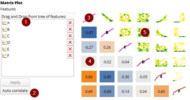
Feature selection area: Drag numerical features from the Feature list to this dialog box.
Auto-correlate button: Automatically selects the features with strongest correlations to your first selected feature.
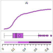
The diagonal shows the name of the feature and the cumulative relative distribution of values as a line graph
The lower left half shows the correlation between the features named in the diagonal on the same row and same column.
Red has a strongly positive correlation
Grey has no correlation
Blue is strongly negative covariance
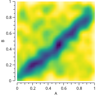
A heat map is a great way of better understanding the form of the correlation between the two features.
XY Scatter Plot
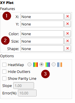
Select features for the X,Y axis
Attribute of color, size and/or shape for each point
Apply modifiers in special cases
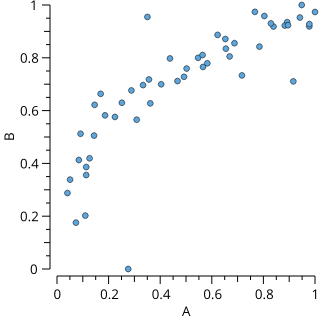
The basic x-y scatter plot will show the points using the color defined for the Y feature.
Changing the color of each point can be useful to find differences between domains.
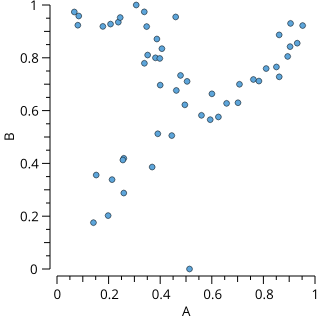
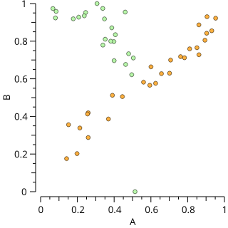
If numerical features are used for color, then the color bins for the feature will be used.
Categorical and numerical features can be used to group points by size or shape.
It is recommended to use size for numerical data and shape for differentiating between categorical data.
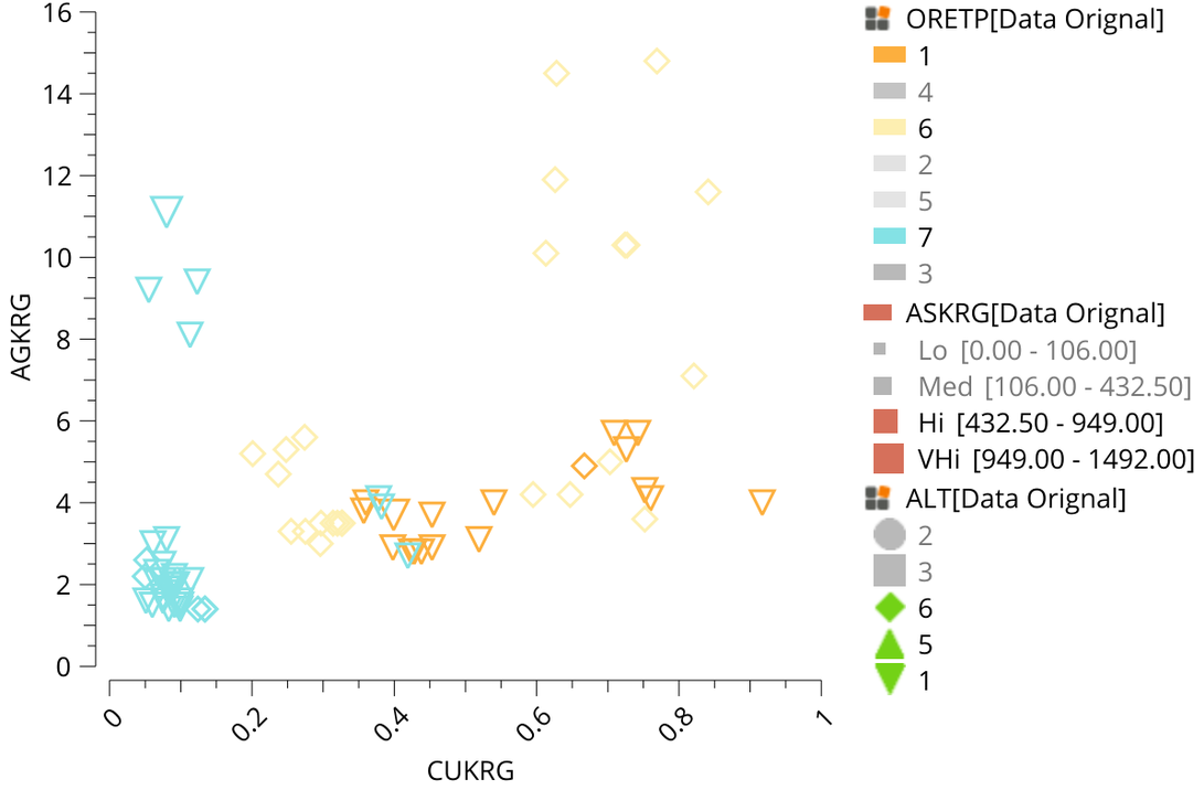
The legend will show the color, size and shapes used, in that order.
Items that were turned off in the Legend window will appear grey in the image that is exported.
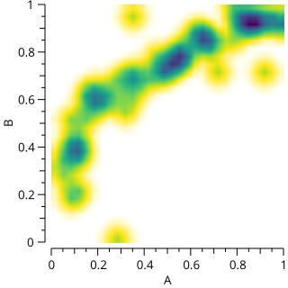
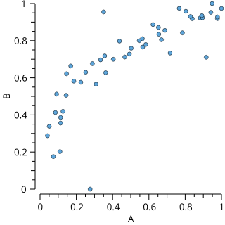
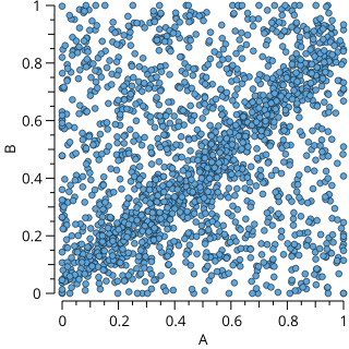
To print the graph, clicking on  icon and the chart will be sent to report, in this window select print on the right side.
The scatter plot shows the relationship between two variables. Each sample is represented by a point in the scatter diagram according to its values for the variables of the X and Y axis. The scatter plots show if there is a correlation between the two variables. A positive correlation is represented by an increase in value in both variables from the origin 0,0. A negative correlation is represented by high values in the variable Y and low values in the variable X. it is also possible that the data are not correlated, showing no discernible relationship.
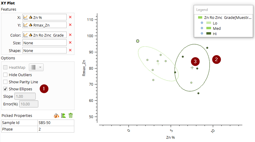
Ellipses
Ellipses are like box-plots in 2 dimensions. They show the 50% confidence interval for a cluster of data.
An ellipse is added for each color grouping of data.
Check the Show Ellipses box.
The ellipse is added in the same color as the data it represents
A cross is added to show the mean for the x and y data features in that group
Data Picker
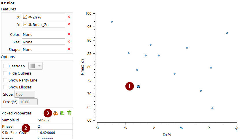
The data picker can be used in the different charts that plot x-y data, such as x-y scatter, ternary diagrams, q-q plots.
Click on a data point of interest (note that it is bigger than the others when selected)
Drag any feature from the Feature List to the Picked Properties box. The values for the selected data point will be shown here.
With the data point selected, use this toolbar to jump to where the sample is in either 3D or Logs view.
Histogram plot
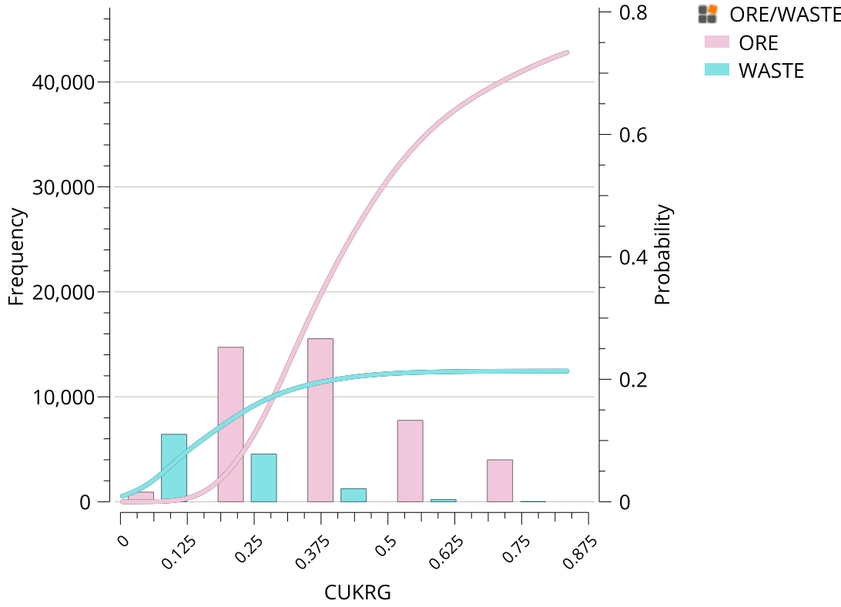
A histogram shows the value distribution of a feature.
The left vertical axis shows the individual frequency of the histogram column bins.
The right vertical axis shows the cumulative relative frequency, represented by the smoothed lines.
If grouping is used, then there are five bins, otherwise there are ten bins for a single feature.
Ternary plot
A ternary diagram shows the relationship between three numerical variables. It is essentially just another x-y scatter plot, but the ratio between the numerical values for each score determines where the score is plotted in the triangle.
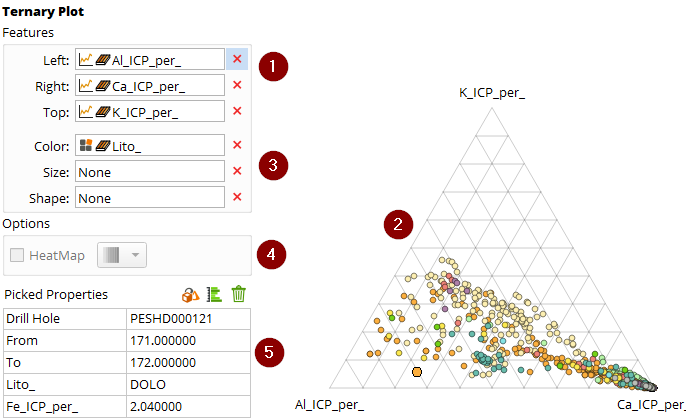
Assign the Left, Right and Top variables
In this example, the axis to the left shows the intensity of K relative to Al and Ca. There are many samples that are dominated by Ca, only a few have much K.
The values can be grouped by color, size and shape, just like an x-y scatter graph.
Unless the values are grouped, a heat map can be generated.
Properties of picked points can be viewed by dragging features to this area.
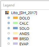
As with other tools in Cancha, the Legend is interactive. Use the radio buttons to turn on and off different categories.
Box Plot
The box diagrams are very useful to compare batch of data and show the distributions of attribute values.

The median is the vertical line within the box.
The average (mean) is the diamond.
The interquartile range (25th percentile to 75th percentile) is the box.
The whiskers represent the limits of 1.5 x the interquartile range.
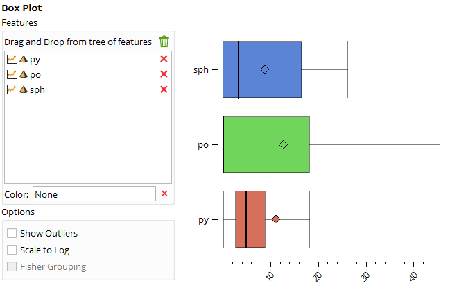
Without grouping, several features can be compared at the same time.
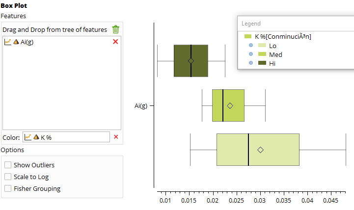
Grouping by categorical data, the colors will be displayed in the legend, per the grouping criteria. If more than a couple of features are grouped by categories then the box plot can get very crowded.
Showing the outliers is possible, but q-q plots are better at showing outliers. Scale to log is useful where different features may be in different orders of magnitude, such as Fe in ppm and S in %.
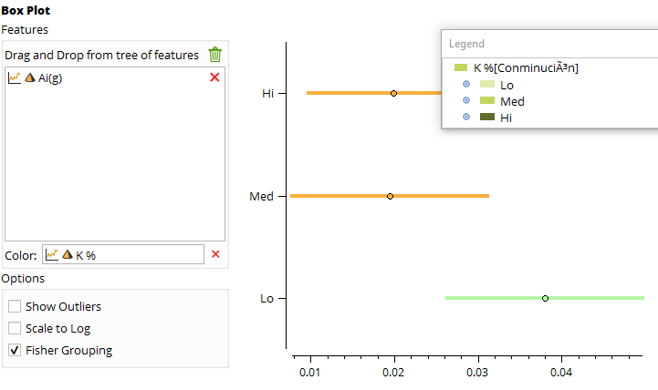
Fisher Grouping
Fischer grouping is an option in the Box Plot tool that is useful to see if certain categories are statistically separate, or if they can be joined to simplify grouping, concentrating the number of samples in fewer domains.
In this example we see that the abrasion index is statistically similar for the high and medium K grade ranges, but significantly different (and higher) in the Low % K range. This can be seen as by the colors used once the Fischer Grouping option is checked.
Distribution Plot
The Distributions chart displays the value distribution of discrete or continuous attributes.
This is useful to see how a small number of sample grades compare to a large set of comparable grades in a block model, for example.
In this example the zinc grade in the block model is represented by the line, and the zinc grade of the metallurgical samples is represented by the dots.
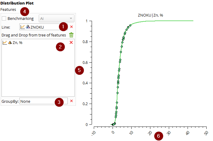
Choose the data to use as the line
Choose one or more data to use as the dots
If just one feature is selected as dots, then you could group the data. For example, by phase or by oretype
Cancha includes benchmarking data curves that can be used as lines for some global data sets for popular comminution parameters.
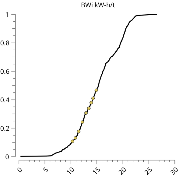
The y-axis is the probability of each value
The x-axis is the value range. In this case most blocks and all samples are less than 10% Zn.
In this example we use the WiBM benchmarking to see that our BWi results are soft to medium, compared to other mines.
Ratio Chart
A Ratio Chart is a useful way to see how the ratio between different numerical features varies throughout the dataset.
Click on the Ratio Chart button
Drag numerical features from the Feature List to this box
The x-axis is the count of values.
The y-axis shows the ratio of the values in each data point, ordered by the first feature in the list.
The title shows the feature names, from bottom to top
In this example, the sulfur area is green and the iron area is yellow.
About 100,000 blocks in this model have ratios of Fe/S of over 5/1. The block with the lowest Fe/S ratio (on the right), has about 2:1 S:Fe, but overall it looks like 80% of the blocks have a S:Fe ratio of about 0.54:0.46, which is pyrite.
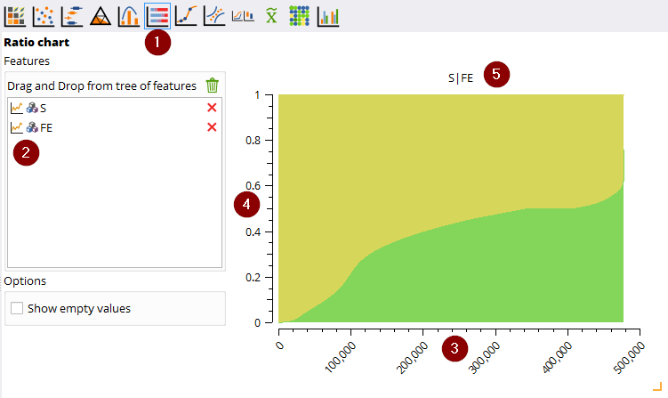
This graph can be useful to see how credit elements or penalty elements vary in the blocks, samples or drill intervals. For example As/Cu, or Cu/Au ratios. The graph supports as many as six variables.
QQ Plot
This tool shows the QQ-plot (or quantile-quantile plot) that compares a feature to either normal or Weibull distributions.
In a QQ plot where the X-value represents the theoretical quantiles from a standard normal distribution (or normal scores) and the Y-value represents the sample quantiles, you are essentially assessing the normality of your data set. Here’s a more specific interpretation based on that setting:
If the data points follow a straight line, it indicates that your data is normally distributed.
The slope of the line will be equal to the standard deviation of your data, and the intercept will be equal to the mean of your data.
Deviations from straight line:
A curvature away from the straight line can indicate skewness in your data.
A curve concave up may indicate positive skew.
A curve concave down may indicate negative skew.
Divergence at ends:
If the points diverge from the straight line at the ends, it indicates that your data has heavier or lighter tails than a normal distribution.
Divergence above the line indicates heavy tails (more extreme values than expected).
Divergence below the line indicates light tails (fewer extreme values than expected).
If the slope of the points is steeper or flatter than the 45-degree line, it suggests a difference in variance compared to a standard normal distribution.
The intercept of the line with the Y-axis can give you an indication of the mean of your data compared to a standard normal distribution (which has a mean of 0).
Any systematic deviation from the straight line suggests that the data distribution is not normal. It could be an indication of a different distribution or the presence of outliers.
Random deviations from the straight line may be due to sampling variability, especially if the sample size is small.
Outliers may appear as points that are far away from the straight line, and can significantly affect the interpretation of the QQ plot.
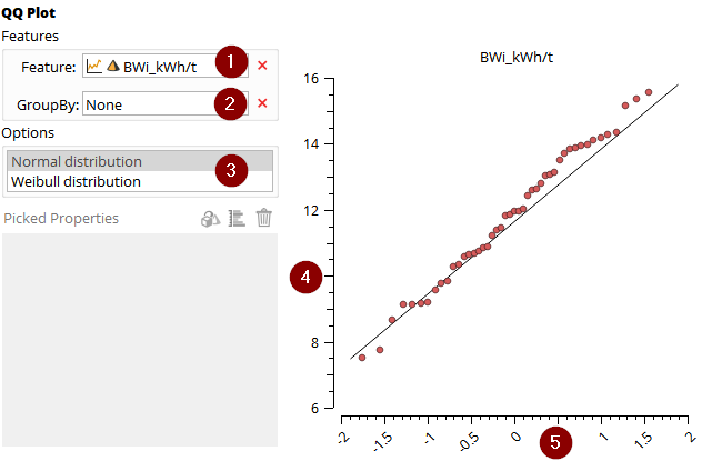
Choose any numerical feature
Group by any numerical feature’s ranges, or by a categorical feature
Choose Normal or Weibull distribution
The y-axis is the feature value
The x-axis is the distribution score
Drag features to the Picked Properties box to investigate points of interest.
Summary Statistics
You can build a table of summary statistics for the numerical features that you choose. Drag the numerical features you want from any table in the Feature List, to the statistics table on the right. To delete a column, double-click its header.
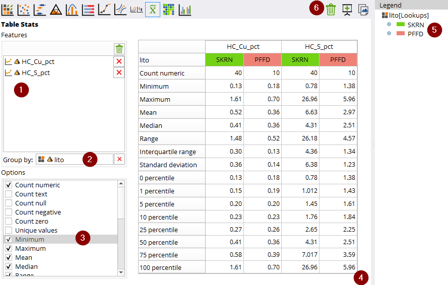
Add the features to be summarized
Add the feature that the summaries should be grouped by
Choose which statistics to be included in the table
Move the scale tool to size the table
The legend can be used to filter what is shown in the table
Clear the table, send an image to Reports, or copy an image to the Windows clipboard
Mosaic Plot
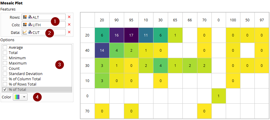
The mosaic plot is useful for displaying the relative density of data in two dimensions.
The same as a heat map for x-y scatter numerical plots, the mosaic plot gives you binned data arranged by discrete categories in the rows and columns.
Choose the categorical features for the row and column headings, like for a pivot table.
Choose the numerical data feature to use
Choose the summary type to display for the selected data
Choose the color scheme that you like
Note, the order that the rows and columns are in are the same order that they appear in the legend editor.
Multi Histogram Plot
The multi histogram plot gives you the relative frequency of a numerical or categorical feature between one or two categorical features.
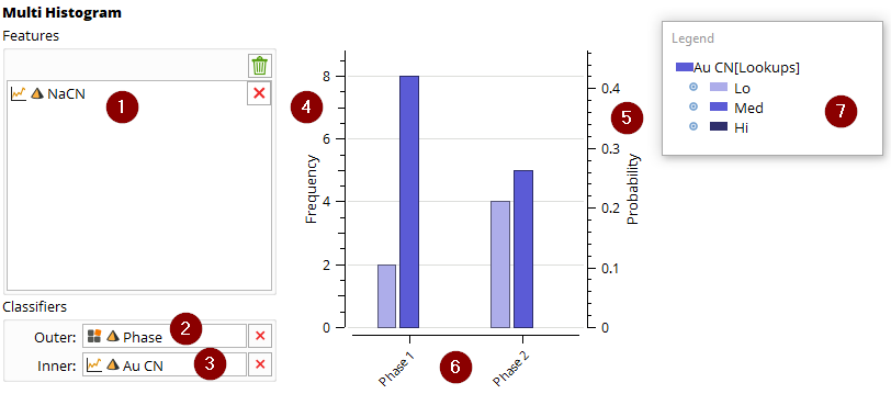
Add the features to be analysed here
The outer classifier is the one that groups the bars on the x-axis
The inner classifier is the feature that groups the sub-population within each outer classification bin
The frequency, or count, of scores in each bin is shown on the primary y-axis
The probability, or fraction of the total, is shown on the secondary y-axis
The outer classification bins are shown on the x-axis
The inner classification bins are shown in the legend.
This multi histogram chart is useful for showing the relative proportions in two systems of categorical domains simultaneously. The mosaic plot does the same thing, but in a different format.
Bias Chart Plot
The bias chart is used to show the relative values in alphabetical order for a data set.
These can be useful for detecting bias between phases of testwork, for example.
In this example, we see that the Phase 2 of testwork was more variable and gave on average much lower recovery values compared to Phase 1.
This chart can only be used for metallurgical data, as there is not enough space for massive data from drilling or block models.
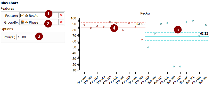
The metallurgical numerical feature to be analysed
The grouping criteria
The error bar 10 of the average to be shown (+/-)
The Phase 1 data shown has an average of 84.45% RecAu and the data is generally inside the 10% error from that average.
The Phase 2 results have an average of 68.32% RecAu and most of the data is well outside the 10% error range.
Stacked Chart
The stacked chart is used to show the relative values of complementary values in a set of metallurgical samples.
These can be useful for detecting relationships between several values and a result.
Stacked charts are commonly used for comparing diagnostic leach components, mineral assemblage or liberation categories between metallurgical samples.
In this example we see how when the ratio of S to Au is high, the gold extraction is low.
This chart can only be used for metallurgical data, as there is not enough space for massive data from drilling or block models.
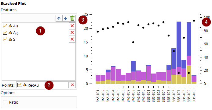
Drag numerical features from a metallurgical sample table for the column data
Drag a numerical feature from a metallurgical sample table for the dot data
The values corresponding to the column data are given on the primary y-axis
The values corresponding to the dot data are given on the secondary-axis
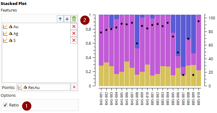
Choose the Ratio check button
The column data is now shown as a relative fraction of the sum of each sample on the primary y-axis
Resources Table
The resource table is a tool that helps to understand how the sample population and domains are related to tonnage and grade in the block model.
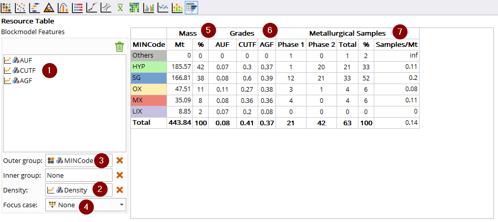
Choose the elements of interest
Choose the density feature, this is the in situ bulk density
Choose a grouping. Examples could be geomet domains, lithology, rock type, alteration, or minzone.
Choose the the focus filter (optional)
Mass estimated for each domain
Average grades for each domain
Distribution of metallurgical samples for each domain
Pivot
Pivot is a tool that summarizes and sorts the tabular data in bins.
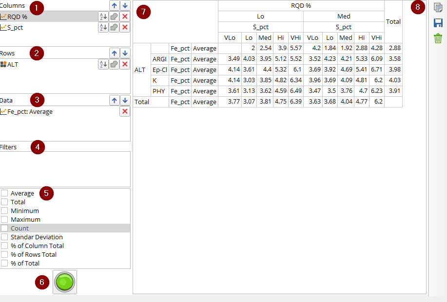
The user can define any of the following by dragging features from the Feature List to the corresponding box:
Columns
Rows
Data
Filters

Features from different input tables can be used, but care should be taken interpreting the results. Irregular data intervals are regularized between tables and resolution is lost. This is similar to how data is transformed between drilling and block models.
Once features have been added to the pivot table, they can be manipulated as required:
Grouping
 Ungrouped, a row or column for each unique value
 Grouped, a row or column for each range or category in the Legend editor
Order
 Sort the table by this feature, in ascending order
 Sort the table by this feature, in descending order
Layer
 Promote the feature to a higher layer. The higher
 Demote the feature to a lower layer
Delete
 Remove the feature from the pivot table
Drag in one or more features for the columns to be used, or leave it empty
Drag in one or more features to be summarized.
Filters can be used to reduce the data to be included. Care should be taken as filtering data from different tables can result in unexpected results.
With the Data feature selected, choose which kind of statistical summary to be included in the table. Multiple statistics can be shown in the same table.
Average is the numeric average of the data in each bin. Interval lengths, rock density and other factors that could influence the average are not considered
Total is the sum of all of the values in each bin.
Minimum is the minimum value in each bin.
Maximum is the maximum value in each bin.
Count is the number of values in each bin.
Standard deviation is the standard deviation of the values in each bin.
% of Column Total is the sum of the values in each bin divided by the sum of all of the values in the column, multiplied by 100.
% of Row Total is the sum of the values in each bin divided by the sum of all of the values in the row, multiplied by 100.
% of Total is the sum of the values in each bin divided by the sum of all of the values in the table, multiplied by 100.
Samples
Cancha has a number of tools that help select samples and composites for metallurgical testwork.
Remember, proposed samples and composites have green icons, executed samples and composites have brown icons.
Definitions: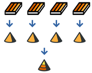
Sample - A metallurgical sample is a single interval of drill core from a single drill hole.
Composite - A metallurgical composites are blends of different samples.
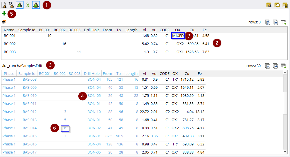
The toolbar has the following options:
 Turn the sample table view on and off
Turn the composite table view on and off
 Export different kinds of tables:
Samples table. This is the table shown in point 3.
Consolidated table. This is the joined table that includes all of the
Drilling tables, using the smallest number of rows while keeping the precision of the original dataEquiInterval table. This is a table that converts the
Drilling tables into a single table with intervals of 1 m. Precision is lost, assumptions are made, sometimes words are said in anger.
Show sample statistics table. This is similar to the same function in Analysis
The
Composites table shows the name and mass of each composite on the left in blue, and a summary of numerical and categorical features on the right.The
Samples table shows the sample name and origin on the left in blue, and a summary of numerical and categorical features on the right.Drag features from the Feature List to this area to add these columns to the analysis.
 New composite. Click this button to add a new composite to the table. Cancha will automatically name the new composite using ABC-XXX:
A is the first letter of the project
B represents the phase (A is 1st phase, B is second phase)
C is for composite (as opposed to S that is for sample)
XXX is the number of the composite in the phase
Cancha will also add columns to the left for each composite. This column shows the weights (or length) that will be used.
In the composites table, the total mass for the composite is shown.
In the samples table, the mass for each sample to be used in the composite can be added directly. Each time a new sample mass is added, the composite table is recalculated.
The summary information is not precise.
- Numerical features are weighted averages by length and other factors like density are not considered.

- Categorical features are summarised based on the most frequent category in a sample, but sometimes the less frequent intercepts are important too. A family of four has a pet elephant. On average they are human, but don’t use that summary when organizing transport.
Be careful and review!
Sample Representivity Report
To compile the formal data metrics and distribution overlays for your independent audit trail, use the Sample Report in the Samples area.
Follow this step-by-step sequence to fill out the configuration form and execute the report:
Open the Configuration Form: Within the Samples area toolbar, click on the Sample Report tool icon to display the properties dialog menu.
Assign the Focus Case Filter: Click the Case Filter dropdown menu at the top of the form and select your target resource case or operational scenario filter (e.g., your saved pit shell or ore zone boundaries).
Select Active Testwork Phases: Under the Select Phase pane, tick the checkboxes for the specific metallurgical testing campaigns that you want to audit against the global resource block model.
Populate the Evaluation Features: Drag and drop your targeted geological, geochemical, or physical driver features directly from the main Feature List into the Features window.
Establish Priority Hierarchy: Highlight features within the list box and use the blue Up ($\uparrow$) and Down ($\downarrow$) arrow keys to arrange them in order of geological or metallurgical priority.
To remove a feature: Click the orange X icon next to the individual feature name, or select the feature and click the green Trash Can icon to clear it.
Generate the Report Dashboard: Click Apply at the bottom of the form.
Cancha will immediately cross-examine your phase testwork data against the filtered block model criteria and update your Samples area with the complete interactive investigation dashboard. This will display multi-directional 3D location views, localized drill log links, and outlier box plots for your reporting checklist.
Sample Selection
Cancha features an integrated machine learning algorithm designed to eliminate the manual, multi-week headache of picking core intervals. By analyzing your complete drilling database against a targeted resource profile, it automatically optimizes the selection of truly representative metallurgical samples. This workflow reduces stakeholder approval lead times, minimizes testing costs, and maximizes statistical confidence.
Core Nomenclature & Concepts
Before launching the selection engine, ensure you are familiar with the foundational criteria used by the algorithm:
Representivity: The extent to which a sample displays the exact same characteristics as the broader resource it is intended to represent in a specific metallurgical test.
Focus Case: The subset of the resource data that you want your samples to physically match. In practical terms, this acts as a global database filter (e.g., "only material inside the year 1–3 pit shell" or "only oxide zones").
Sampling Frame: The drillings where the samples will be taken from. Often limited to holes that were diamond drilling, or recently drilled, for example.
Principal Features: The specific geological or geochemical factors that directly drive your process targets (e.g., Lithology, Alteration, and RQD for comminution; Mineralogy and Clay content for flotation).
Step-by-Step Sample Selection Workflow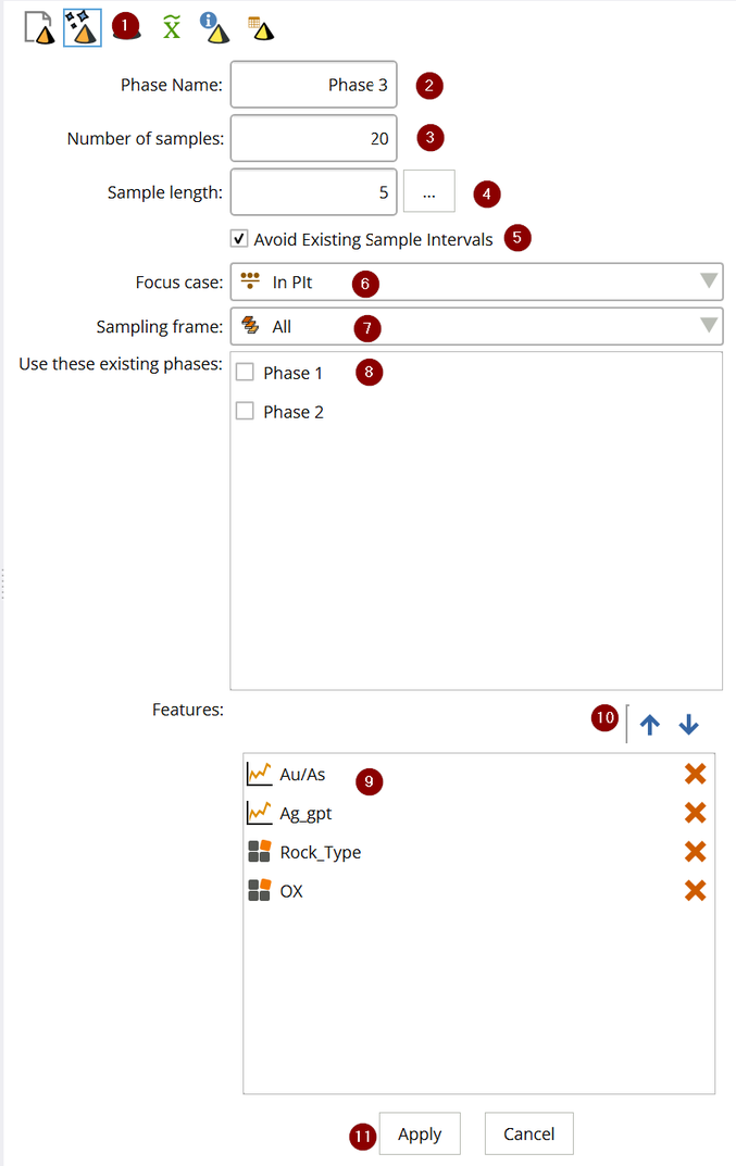
Follow this step-by-step sequence to run a sample selection campaign.
Navigate to the Workspace: Samples area from the main top toolbar:
Launch the Interface: Click on the Sample Selection tool icon within the contextual toolbar.
Set the phase name for the new phase.
Set Sample Quantity: Choose the total number of samples required for your laboratory program.
Rule of thumb: Advanced variability programs typically require a minimum of >30 samples per domain or >150 samples total for late-stage projects.
Define Interval Length: Specify the target length for each sample interval. This length should reflect your mineralization intercept and minimum mining cut (e.g., your operational bench height) to maintain practical utility. The button to the right gives you a calculator for interval length from mass and drillcore diameters.
If you want to avoid re-sampling the same core, check the bock to avoid existing sample intervals.
Assign the Focus Case: Select your target focus case directly from your pre-defined filter case dropdown menu.
Troubleshooting: If your focus case dropdown is empty, you must jump to the Filters area first to establish and save your case criteria.
Set the Sampling Frame: Select the explicit list of drill holes available in your core shack from which the software is permitted to pull material.
If you want the new samples to fill in the representativity gaps from previous sample phases, check them here.
Identify Driver Variables: Choose your target Principal Features from the active Feature List.
Establish Feature Priority: Drag these features into the priority pane and order them sequentially from highest to lowest impact.
Execute: Click Apply.
The engine will execute immediately, extracting a candidate population of representative core intervals and displaying them as green "proposed" intervals within your workspace.
The Representivity Audit
Once Cancha generates your sample suite, navigate directly to the Analysis workspace to audit its work. Use the Distribution Plot to overlay your sample population against the entire block model:
The Line represents your total resource distribution.
The Dots represent your newly selected metallurgical samples.
An optimized selection will show the dots tracking the range of the curve of the line across all categorical histograms and numerical grade ranges, supporting representativity with respect to these features..
Forming composites
Cancha does not have a way of importing composites yet, but you can declare the composites in Cancha once you have the samples declared or imported.
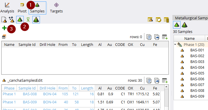
Go to Samples area
Click on the sample button to bring up the same table
Click on the plus sign at the top of the Composites box.
It does some consolidating, so wait a few seconds. You’ll get a new composite in your composite list.
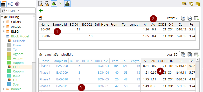
Each time you click the plus you get a new composite and a new column opens up in the samples table
Drag the features that you want to summarize from the Feature List to the summary table on the right.
In the empty composite columns, manually type in the quantity of each sample in each composite. It’s dimensionless, but we assume that it’s mass.
The weighted average is given for numerical values (Al,Au,Cu and Fe in this example), and the most abundant value is given for categorical values (Ox and CODE in this example)
Viewing samples and composites
Once your samples or composites have been imported or declared, you can visualize them in 3D.
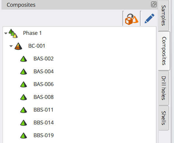
In the 3D view area go to the Samples tab or Composites tab on the far right of the screen.
Click on a phase, a composite, or a sample and it will be highlighted in the 3D area. Note that if you have not selected a valid feature from your metallurgy features in the Feature List, nothing will show up.
You can color the samples by any numerical or categorical feature that you have in metallurgy, such as grades, phase, alteration, etc.
Note that composites are not highlighted in the Logs view, if you need to do something like that, then export the composites table, then import it again as a feature of each sample.
Sample Classifier
Use any features from Metallurgy to classify the samples into bins.
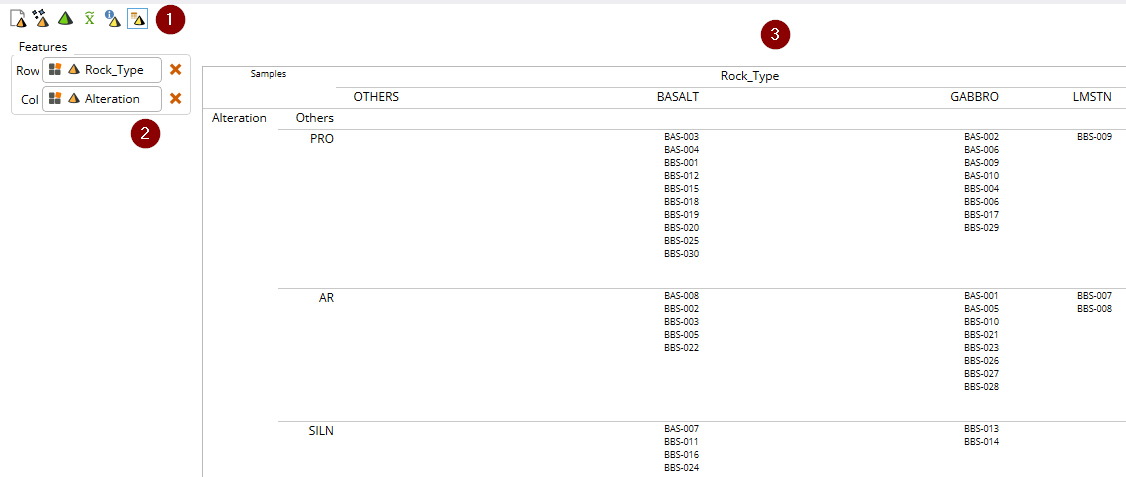
Sample Report
Click on any sample in 3D, Analysis, or Targets, and you can open a Sample Report in the Samples Area.
The following is given in this investigation dashboard:
Sample name and drill hole ID
The features that were detected automatically as being those where this sample is an outlier
You can also add other features such as principal features or targets as you prefer
A table of the values of these features is given
The location in 3D, showing the Northerly, Easterly and plan views are given
The box plots show the values of the sample population, and the black dot is the sample in question.
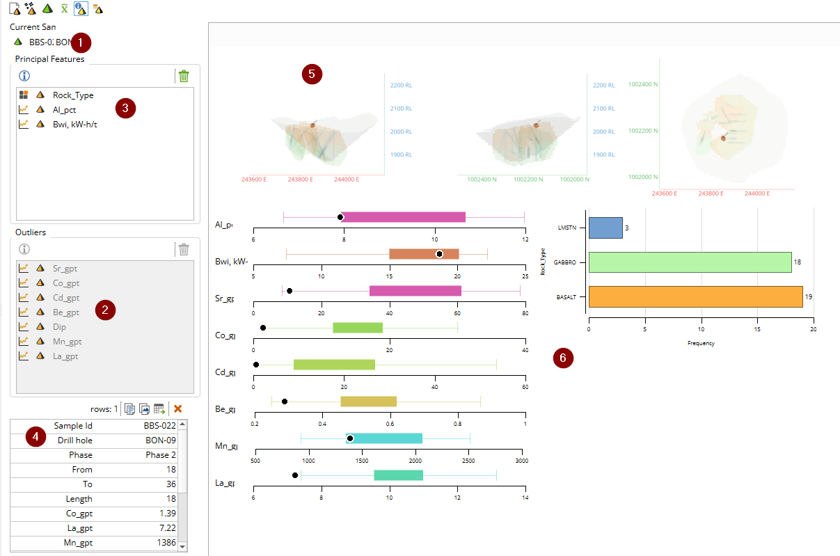
Targets
Inside Cancha there is a machine learning algorithm we call Canchita.
Canchita takes the imported features, the derived features, the interpolated features and evaluates how each of them relates to a Target.
There are two major mechanisms by which Canchita improves the precision in predicting a Target:
Diving the data into separate domains that behave differently, using categorical features, or binned ranges of numerical features. This is by far the most popular and most successful method.
Generating regression formulae that relate a numerical target to numerical features.
Domains
All features are considered by Canchita to be possible domain classifiers.
Categorical data, such as rock-type or stope are ready to go, but it is still important to run some feature engineering to help Canchita find results. For example, if you know that there are 12 lithologies mapped, but they can be grouped adequately into just three groups, such as “sedimentary”, “volcanic”, and “skarn”, then do that. The fewer categories that are considered, the more samples there are in each category and the better the chance of finding something statistically interesting. Remember not to combine things that are different.
Ranges of numerical data are also categorical, as the continuous numerical values are also grouped into ranges. A great start can be to have the three ranges, for example:
Waste is below cut-off grade
Nominal is typical mill feed
HiGrade is over the maximum average mill head grade
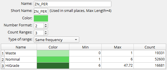
Other tactics can be in bins of such as:
Concentrate quality (Hi/Lo As, Hi/Med/Lo Au)
Geochem ratios (Fe/S, Zn/Cu, Au/Te)
Regression formulae
The most popular form of a regression formula is recovery vs head grade. In our experience, this only works in a small fraction of studies, but it is expected in every study.
Running Targets
The Targets workflow involves three main steps:
Select your target metallurgical parameter
Choose predictor features
Review and select the best models
This process typically takes 2-10 minutes depending on data size.
Choose your Target
Declare which target you would like to get models for.
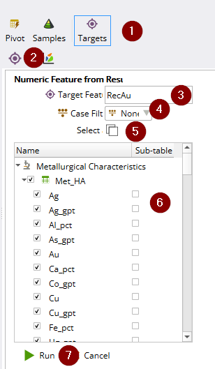
Go to the Targets area
Choose the Target tool
Drag the Target feature from a Metallurgical Results table
Cancha will automatically ignore other results, header features
Choose select all, or not. Cancha can consider all Characterization features including those projected from drilling and block models. Also, Parameter features and Origen features can be used for predicting Results too.
If some features don't have full coverage, then they will create a subtable. To force a sparsely populated to be considered as a predictor, check it for the subtable
Run the algorithm, it can take a few minutes for large data sets.
Once you have worked out which features you would like to use, run the algorithm.
When you are getting started, it is good just to let it run with all of the data possible. It only takes a few minutes to run, and will come up with some crazy relationships, but some may be so crazy that they are actually confused with genius.
Reviewing Models
Thousands of models are considered by Cancha, but it only presents the models that it considers to be interesting.
There are four kinds of models that are shown:
Recommended models - Models that exceed in the precision, accuracy, parsimony and ranged statistical criteria that we have established.
Supported models - Models that are statistically suitable, but does not meet our demanding requirements
Supported non-linear models - Models such as logarithmic, exponential and other non-linear models that are not easily subjected to the scrutiny of the Cancha model selection process. They are presented with just the r² indicated, and the analyst can decide if they are useful or not.
Extra models - Models that may be helpful for further investigation, but should not be used for inputs to mine planning.
There are always constant models (e.g. BWi = 13.5 kW-h/t).
Linear models (Y=a+bX) and non-linear (Log, sin, ex, etc) are only shown where appropriate.
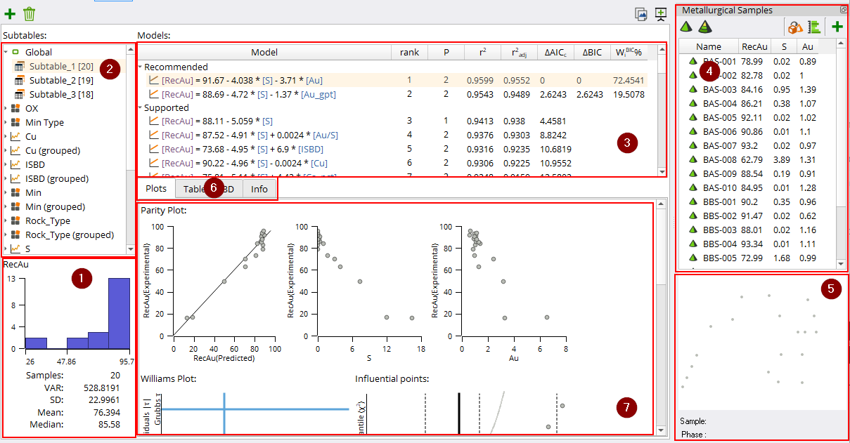
The target model result window has a lot going on, but do not be intimidated.
Summary data for the Target which has been analysed is shown
The domain system that is selected
The list of models found by Canchita for the domain selected in the selected domain
The sample list showing the Target and the model parameters for the each sample for the selected model and domain
An interactive map of the samples locations in plan view
Tabs for model views:
Plots (shown)
Table
Mini-3D views
Info
A series of interactive plots showing the model fit performance, residual analysis and statistics for the selected model, and selected domain.
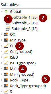
Domain List
The domains in the Domain List is broken down as follows:
Global includes all data points in a single regression model
The number after the domain indicates how many result data points are in that domain.
Numerical data ranges are sometimes proposed as domaining systems.
Categorical data is also a potential basis for domain selection
Where statistically significant, grouped ranges and categories are grouped into simplified domains, increasing the population size in each domain, and reducing the chance of overfitting models.
Model List
The more samples you have in a domain, and the more features that are available for analysis, the more likely it is that Canchita will find a few models to choose between.
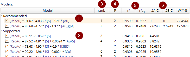
The model list has the following aspects:
Recommended models. In theory they are superior models, just check they make sense geometallurgically!
Other models are included:
Supported non-linear models, includes exponential, logarithmic transformations
Supported linear models. These are interesting to review, but do not use while under the influence of alcohol or sleep deprivation. See which features they picked up and use them as a basis for further investigation.
Extra models. These are the mean and median values for the domain section. They never let you down.
Only interesting models are shown. Canchita tests thousands more models, but only shows those that are recommended in the Model List.
Models are ranked from most recommended to least.
P = the number of parameters in the model
r² and r²-adj are indicators of how well a change in parameters match the corresponding change in target values. Numbers closer to 1 are better.
These parameters are in part indicative of overfitting. Where there are a large number of potential parameters, and few Results, parsimony is very important to consider. Cancha has considered these when ranking the models, and choosing how many parameters are appropriate.
Target Summary Stats
This window shows a summary of the target input data that was analysed in the subtable used. It is not affected by the predicted values.
| Samples - Number of samples |
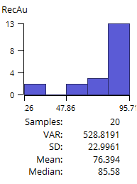
Williams Plot
The Williams plot is a very powerful diagnostic tool for improving confidence in model selection.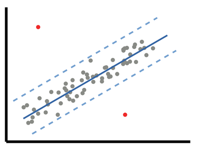
The Studentized values on the vertical axis describe the extent to which each point is likely to be a member of the same set of data as the other points. High values are otherwise known as outliers. Outliers on this graph are normalized, so it could mean that the sample has an unusually high, or low value, compared to the other samples in the analysis.
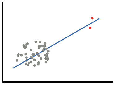
The leverage values on the horizontal axis describe the amount of influence each sample has over the final result, compared to the samples. If a point has high leverage, then a change in that point would have a high impact on the model parameters. This can be a sign of mixed domains, lack of sample density, or data errors.
Both outlier tests and leverage tests are not intuitive on simple x-y plots where multiple parameters are used in the regression.
The combination of the outlier and leverage analysis on a single Williams plot facilitates the regression diagnosis, identifies risks to be investigated, and brings higher confidence in model selection.
| Points in the lower left quadrant support the model well |
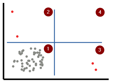
The blue lines on the Williams plot are the threshold lines that have been drawn subjectively based on Transmin’s experience. They are not hard and fast lines, but are useful for guidance.
Interaction with the Metallurgical Samples List
Click on a model and the Metallurgical Sample List will be populated with the list of samples in the subtable that were used for the model.
In this example, the selected model uses Ga and U grades to predict RecAu.
The Metallurgical Sample List was populated with the samples, and the corresponding target and predictor values for each sample.
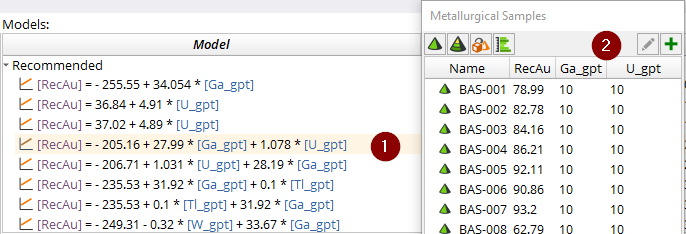
Clicking on these elements will highlight the same element in the other windows:
Metallurgical sample list item
Any of the model report plots
The metallurgical sample mini-map
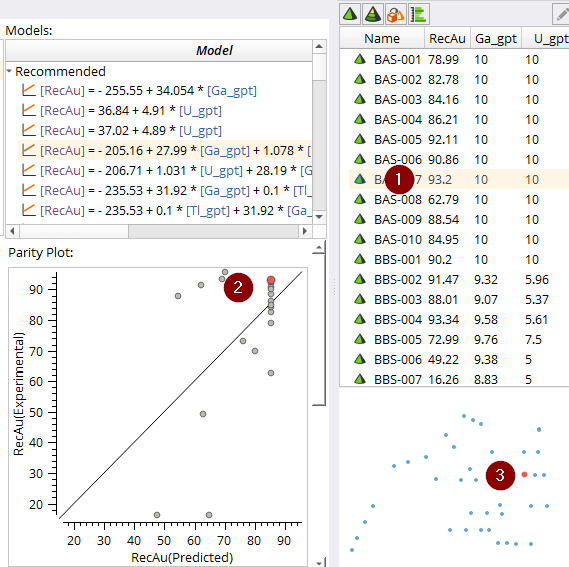
If the second screen 3D window is open, clicking on any of these items will also automatically highlight the same sample in the 3D window.
Jumping to the selected sample in 3D or Logs can also be achieved by click on the button in the Metallurgical Sample List toolbar.
Domain Trees
Domain Tree is a decision tree analysis tool that groups samples with similar metallurgical characteristics using sequential decision nodes. Each node represents a specific criterion that divides samples into subgroups based on their metallurgical behavior.
Workflow:
Drag your target feature from the metallurgical results table
Apply a case filter if needed (created in the Filters interface)
Select features to include in the analysis - use "Select All" or choose specific features
Choose a sub-table option to focus on samples with complete data for your selected characteristic
Run the algorithm
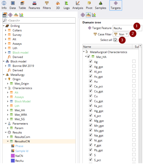
Case Management: Cancha generates multiple decision tree cases based on data quality:
Cases 1-3: Include outliers with different null value handling
Cases 4-6: Exclude outliers with different null value handling
Each case eliminates either columns or rows with missing data, or retains only complete datasets. The following table describes each case in detail and the name assigned.
Case | Name | Description |
Case 1 | “111” | Includes outliers. Eliminates columns with at least one null value |
Case 2 | “110” | Includes outliers. Eliminates rows with at least one null value |
Case 3 | “100” | Includes outliers. Does not contain null values |
Case 4 | “011” | Exclude outliers. Eliminates columns with at least one value null |
Case 5 | “010” | Exclude outliers. Eliminates rows with at least one null value |
Case 6 | “000” | Exclude outliers. Doesn’t contain null values |
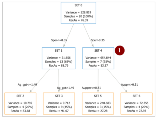
Tree Interpretation:
Blue nodes: Decision nodes that can branch further based on threshold values
Orange nodes: Terminal nodes providing final predictions
Each node (SET 0, SET 1, etc.) displays statistical summaries including variance, population, and mean
Click blue nodes to see threshold analysis graphs
Parity plots compare predicted vs experimental values
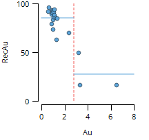
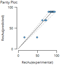
Application:
Use decision trees to identify clear metallurgical domains based on measurable characteristics. The tree structure reveals which features most effectively separate samples with different metallurgical behavior, supporting domain-based geometallurgical modeling.
Principal Component Analysis (PCA)
PCA is an unsupervised clustering technique that groups similar materials based on selected features. It's most effective when applied to focused feature sets rather than general geochemistry.
Workflow:
Choose your data source: Drilling, Block Model, or Metallurgy
Select the features you want to include in the analysis
Click Run
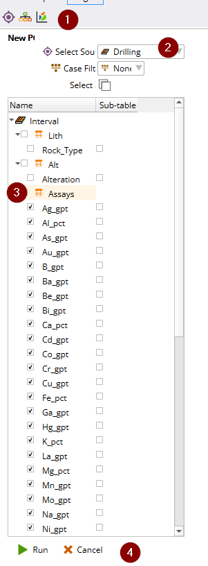
Cancha will present three clustering options:
K-means clustering - partitions data into distinct clusters
Ward clustering - hierarchical approach that minimizes variance within clusters
GMM (Gaussian Mixture Model) - probabilistic clustering that allows overlapping clusters
Evaluating Results: Box plots display the grade ranges for each selected feature across all clusters for each clustering technique. This helps you compare how well each method separates your data.
Clusters are automatically named based on the features that most strongly influence each cluster's characteristics.
Implementation: Select your preferred clustering technique from the results and click Apply. A new categorical feature will be created in the "Derived" table in your Feature List.
Application: Use this new categorical feature in 3D visualization and Logs to:
Identify what geological events or processes the clusters represent
Evaluate potential for geometallurgical domain generation
Remember: if you can't explain the geological meaning of your clusters, the analysis may not be useful for geometallurgical modeling.
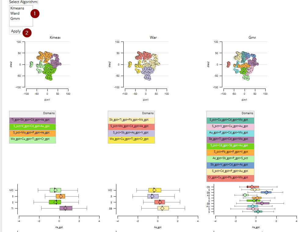
Installation and Activation Procedure
The installation and deployment process ensures successful deployment.
Download the Installation File: The software is downloaded from www.cancha.pe .
Run the Installation Executable: Follow the prompts to install the core application files.
License Activation: The software requires activation through the online license management service.
An Activation code is provided by Transmin, usually by email.
Activation typically occurs instantly during installation.
Ensure your system is allowed to connect to the license management service for activation, renewal, and continued functionality.
Network and License Activation Requirements
Cancha geometallurgical software utilizes an online license management service for activation and validation. An Internet connection is mandatory for this periodic process and for software updates.
For systems operating behind a firewall or restricted network, the client's support staff must ensure that the following network protocols and ports are open and accessible to allow the Soraco QLM license management service to function:
Protocol | Port Number | Purpose |
HTTP | 80 | Used for initial license communication and validation. |
HTTPS | 443 | Used for secure license communication and validation. |
The Soraco QLM License Management service collects the license identifier and computer identification for activation purposes. Transmin confirms that no project data or personal information is collected or accessed through this service.
If the connection is successful, the software receives its time-limited and machine-limited license keys. If the license is deactivated (e.g., due to connectivity failure or remote deactivation by Transmin), the software will remain installed but will not operate until re-activated.
Crashes
Cancha is a complex software, and occasionally it will crash. There are errors that users can make to cause a crash, and there are oversights from the development team that can cause crashes too.
Preventing Data Import Errors
Proper data preparation before importing into Cancha prevents crashes, analysis errors, and incomplete results. The most common cause of Cancha crashes is importing numerical data that contains text characters. Follow this checklist to ensure smooth data import and reliable analysis.
Critical Data Cleaning Requirements
Numerical Data Must Be Purely Numeric
Cancha will crash if numerical columns contain any text characters. Common problematic entries include:
Remove these from numerical columns:
Detection limits: ">1%", "<0.01", "≤0.5"
Null indicators: "N/A", "NULL", "n.d.", "BDL", "---"
Text annotations: "1.5*", "2.3 (est)", "pending"
Unit labels: "5.2%", "123 ppm", "15 g/t"
Range values: "1-3", "2.5±0.1"
Replace with:
Empty cells (preferred for missing data)
Empty (Cancha's recognizes null values)
Actual numeric values where appropriate
Example Data Cleaning
Before (problematic):
Cu_Grade | Au_Grade | Fe_Grade |
2.1 | 0.05 | >15% |
<0.01 | N/A | 12.3 |
3.5* | 1.2 | BDL |
After (clean):
Cu_Grade | Au_Grade | Fe_Grade |
2.1 | 0.05 | 15 |
0.005 | 12.3 | |
3.5 | 1.2 | 0 |
Data Structure Requirements
Header Requirements
Single header row only - Multiple header rows will cause import errors
Unique column names - Duplicate headers prevent proper feature mapping
No merged cells - Excel merged cells break the import process
No special characters - Avoid symbols like #, %, $, & in header names
Table Organization
One data type per table - Don't mix assays and lithology in the same table
Consistent units - Ensure all values in a column use the same units (don't mix %, ppm, and g/t)
Complete intervals - Drilling data must have valid From/To depths for all records
Recommended Data Preparation Workflow
1. Review Raw Data
Before any cleaning, understand your dataset:
Identify which columns should be numerical vs categorical
Count total records and check for reasonable data ranges
Note any obvious data quality issues
2. Clean Numerical Columns
For each numerical column:
- Find/replace common text patterns (>, <, N/A, etc.)
- Check minimum and maximum values for reasonableness
- Identify and investigate extreme outliers
- Ensure consistent decimal places and units
3. Standardize Categorical Data
Consolidate similar categories (e.g., "QZPX", "QZ-PX", "Quartz Porphyry" → "Quartz_Porphyry")
Limit categories to manageable numbers (typically <12 for effective analysis)
Use consistent naming conventions (avoid spaces, special characters)
4. Validate Data Relationships
Ensure drill hole IDs match between tables (collars, assays, lithology)
Verify From/To intervals don't overlap or have gaps
Check that metallurgical Sample IDs link correctly to drill holes
Common Data Issues by Source
Drilling Data
Missing survey data - At minimum, collar coordinates must be complete
Overlapping intervals - From/To ranges that overlap will cause spatial errors
Inconsistent hole naming - "DDH001" vs "DDH-001" vs "DDH_001" will be treated as different holes
Mixed coordinate systems - Ensure all coordinates use the same projection/datum
Block Model Data
Sub-block models - Regular block dimensions work best; sub-blocks may display incorrectly
Rotated coordinates - Ensure coordinates are in world/project system, not local rotated coordinates
Missing mandatory fields - Must include Easting, Northing, and RL/Elevation at minimum
Metallurgical Data
Inconsistent Sample IDs - Must exactly match between Origin, Characteristics, Parameters, and Results tables
Mixed test phases - Keep different test campaigns in separate tables when possible
Unit confusion - Be especially careful with percentages vs decimals (85% vs 0.85)
Data Validation Checklist
Before importing into Cancha:
☐ All numerical columns contain only numbers, empty cells, or single dashes
☐ Headers are unique and contain no special characters
☐ No merged cells in Excel files
☐ Coordinate systems are consistent across all spatial data
☐ Sample/Hole IDs are consistent between related tables
☐ Units are consistent within each column
☐ Extreme outliers have been investigated and verified
☐ Categorical data has been consolidated to manageable groups
Quick Excel Cleaning Tips
Find and Replace in Excel:
Select the data range for numerical columns
Find: > Replace with: (empty) - removes greater-than symbols
Find: < Replace with: (empty) - removes less-than symbols
Find: N/A Replace with: (empty) - removes null indicators
Find: BDL Replace with: (empty) - removes below detection limit
Check for Hidden Characters:
Use Excel's CLEAN() function to remove non-printable characters that might not be visible but will cause import errors.
Validate Numeric Columns:
Use Excel's ISNUMBER() function to identify cells that appear numeric but contain hidden text.
When Import Still Fails
If Cancha crashes during import despite following these guidelines:
Check the last row imported - The error often occurs at a specific problematic record
Import smaller test files - Try importing just the first 100 rows to isolate the issue
Export from Excel as CSV - Sometimes Excel formatting causes issues that CSV export resolves
Check for unicode characters - Ensure text uses standard ASCII characters, especially in categorical data
Remember: Time spent on proper data preparation prevents hours of troubleshooting later and ensures reliable analysis results throughout your project.
Retry
BugSplat
If you encounter a problem that causes Cancha to unexpectedly close, the BugSplat dialog box opens and invites you to send us an error report describing what happened just before Cancha had to close. Please do send us the error report, and please include a description of what happened just before Cancha had to close. This really helps us to track down and fix any problems that cause our software to close. Please be aware that you may not receive a response after submitting a BugSplat.
Troubleshooting
Check out the following common solutions in response to a BugSplat:
Update to the latest version of Cancha
Update the driver for your graphics card
Check your numerical data for text values ☢️
NVIDIA Error
NVIDIA "Unable to recover from a kernel exception."
This error happens when the graphics card is selected for processing but the GPU performance is much lower than the CPU performance. The workload sent from the CPU to the GPU is overloading the GPU.
Solution
Check the driver's version and ensure the GPU is up to date.
Remove the use of the GPU for processing in the processing options:
On the menu bar, click Process > Processing Options...
Select the tab Resources and Notifications.
Unselect the listed graphics card.
Click OK.
Change the graphics card to a model more balanced with the CPU.
ESENT 455 and PERFLIB 1023
Cancha closes randomly.
There is a known bug in Windows, which causes events ESENT 455 and PERFLIB 1023, when this folder does not exist.
C:\Windows\System32\config\systemprofile\AppData\Local\TileDataLayer\Database
If you are experiencing this problem that Cancha closes randomly, consult your IT professional, and ask them if your computer is suffering from the known update bug that causes ESENT 455 and PERFLIB 1023. Adding the missing folders might fix the issue.
End User License Agreement
IMPORTANT NOTICE TO ALL USERS:
BY DOWNLOADING THE SOFTWARE OR ACCEPTING THESE TERMS BELOW YOU AGREE TO THE TERMS OF THIS LICENCE WHICH WILL BIND YOU AND/OR YOUR EMPLOYEES, CONTRACTORS OR REPRESENTATIVES. THE TERMS OF THIS LICENCE IN PARTICULAR INCLUDE LIMITATIONS OF LIABILTY IN CLAUSES 14 TO 16.
IF YOU DO NOT AGREE TO THESE TERMS WE WILL NOT LICENCE THE SOFTWARE AND DOCUMENTS TO YOU. PLEASE DISCONTINUE THE DOWNLOAD OF THE SOFTWARE BY CLICKING THE ‘CANCEL’ BUTTON BELOW AND/OR DISCONTINUE ANY USE OF THE SOFTWARE AND DOCUMENTS.
This licence agreement (Licence) is a legal agreement between you (Licensee or you) and Transmin MC S.A.C., a company incorporated in Peru with registered number 20506197539 (Transmin, Licensor, us or we) for:
beta or commercial release versions of Cancha® computer software and any associated media (Software), and
the release notes made available at the time of release of the Software as available on the cancha.pe website (Documents).
We licence use of the Software and Documents to you on the basis of this Licence. The granting of this licence does not transfer ownership of the Software or Documents to you, which will always remain with Transmin.
Licence: Subject to all applicable terms, Transmin grants you a non-exclusive, non-sub-licensable and non-transferable licence to use the Software and Documents in accordance with this Licence and all applicable technology control or export laws or regulations.
Scope of Licence: You may:
download, install and use the Software on a computer provided by you for your internal business purposes in accordance with the licensing permissions applicable to you;
receive and use any free supplementary software code or update of the Software incorporating “patches” and corrections of errors as may be provided by us from time to time; and
use any Documents in support of the use permitted under this condition 2 and make one copy of the Documents as reasonably necessary for its lawful use.
Restrictions on Use: You must not:
translate, adapt or modify the Software issued to you by us for licensing purposes (Dongle), or do anything to circumvent the operation of the Software, or combine or integrate the Software with any other product;
separate any component part of the Software for use on more than one computer;
lend, rent, lease, transfer, assign or otherwise deal in the Software, Documents or your rights under this Licence without the prior written consent of Transmin;
make alterations to, or modifications of, the whole or any part of the Software, nor permit the Software to any part of it to be combined with, or become incorporated in, any other programs; or
disassemble, decompile, reverse-engineer or create derivative works based on the whole or any part of the Software nor attempt to do any such thing except to the extent expressly permitted by law.
Support: Except where you have a perpetual licence or a licence to use a beta version of the Software, your licence includes the right to receive support services and updates in accordance with the policies and processes published on our website from time to time. If you have a perpetual licence, the receipt of support and updates is subject to the payment of the necessary support fee.
Intellectual Property Rights: You acknowledge that the intellectual property rights in the Software and the Documents are vested in Transmin and that you have no rights in or to the Software or Documents other than the right to use them in accordance with the terms of this Licence. You must maintain all intellectual property notices appearing on the Software, Documents and must not remove the same. You must notify Transmin immediately in writing if you know of any circumstances that suggest that any person may have unauthorised knowledge, possession or use of the Software or Documents. You acknowledge that you have no right to access the Software in source code form.
Confidentiality: From time to time, one of us (Disclosing Party) may disclose Confidential Information to the other (Receiving Party). The Receiving Party must at all times, ensure the confidentiality of the Confidential Information and ensure that its officers, employees and agents do not disclose, communicate, copy or reveal for any purpose whatsoever the Confidential Information except as permitted under this Licence. For the purposes of this clause, Confidential Information includes the Software, Documents, any Dongle(s), information relating to the customer account and any other information provided by Disclosing Party to Receiving Party as confidential, or which from its nature and content is, or would reasonably expected to be, confidential. The obligations under this clause will survive termination of this Licence.
Performance warranty: With respect to commercial release versions of the Software and excluding beta versions of the Software, we warrant that:
the Software will, when properly used and on an operating system for which it was designed, perform substantially in accordance with the functions described in the Documents; and
that the Documents correctly describe the operation of the Software in all material respects, for a period of 90 days from the date of installation of the Software (Warranty Period). Subject to the foregoing, the Software is licensed is provided to you “as is” and all representations or warranties (statutory, express or implied except any which may not lawfully be excluded) are expressly excluded, including any implied warranties of merchantability and fitness for a particular purpose.
If, within the Warranty Period, you notify us in writing of any defect or fault in the Software as a result of which it fails to perform substantially in accordance with the Documents, we will, at our sole option, either repair and replace the Software provided that you make available all the information that may be necessary to help us to remedy the defect or fault, including sufficient information to enable us to recreate the defect or fault.
The warranty does not apply if the defect or fault in the Software results from you having:
altered or modified the Software; or
used the Software in breach of the terms of this Licence.
With respect to beta versions of the Software you acknowledge that the Software is provided on an as is basis without any warranty of any kind.
IP Warranty: Transmin warrants that to the best of its knowledge the Software does not infringe any valid patents, trademarks, copyrights or trade secrets owned by a third party.
IP Infringement: You will promptly provide Transmin written notice if you have knowledge of a claim or the likelihood of a claim by a third party that the Software infringes that third party’s intellectual property rights. If the Software becomes or, in Transmin’s opinion, is likely to become the subject of any injunction preventing its use as contemplated herein, Transmin may in relation to commercial release version of the Software, at its option:
obtain for you the right to continue using the Software; or
replace or modify such Software so that it becomes non-infringing without substantially compromising its principal functions.
If neither 12(a) nor 12(b) are reasonably available to Transmin or the claim relates to a beta version of the Software, then we may terminate this Licence upon written notice to you. Upon return of the Software or written confirmation that it has been uninstalled we will refund to you:
in the case of a licence for a fixed term, a prorated portion of the licence fee paid by you for the then current term (based on the portion of the then current term that would have occurred after the date of termination); or
in the case of a licence for a perpetual term, an amount calculated as the sum of (X) a prorated portion of the Support Fees paid by you for the then current support period (based on the portion of the such support period that would have occurred after the date of termination), plus (Y) the licence fees specified paid by you for your licence amortized on a straight-line basis over a 3 year period from delivery (for clarity, in the case of termination of the licence for a Perpetual Term at the end of the second year, (Y) would equal 1/3 of the original licence fees, and in the case of such termination after the end of the third year, (Y) would equal zero).
Limitation of liability: You acknowledge that the Software operates in a predictive manner relative to input of which Transmin has no control over the collection, use or interpretation, and you agree to accept the entire risk as to the use and the results of the use of the Software in the terms of correctness, accuracy, reliability and performance. Furthermore, you acknowledge that the Software has not been developed to meet your individual requirements, and that it is therefore your responsibility to ensure that the facilities and functions of the Software as described in the Documents meet your requirements. Transmin will not be liable to you under the law of tort, contract or otherwise for any:
indirect or consequential loss or damage,
loss of profits, sales, business or revenue;
business interruption;
loss of anticipated savings;
loss or corruption of data or information; or
loss of business opportunity, goodwill or reputation.
Subject to clause 16, our maximum aggregate liability under or in connection with this Licence whether in contract, tort (including negligence) or otherwise shall be limited to the total amount paid or payable by you for the Software in the 12 months prior to the event giving rise to the liability.
Nothing in this Licence shall limit any liability that cannot be excluded or limited by Peruvian law.
Default and Termination: Transmin may terminate this Licence immediately by notice in writing to you if you breach a material term of this Licence or commit any persistent breach of your obligations under this Licence and fail to remedy the breach within 15 days after notice from Transmin requiring the breach to be remedied. For the avoidance of doubt, material provisions of this Licence include any which relate to what you can or cannot do with respect to the Software and any provisions related to intellectual property rights or confidentiality.
Immediately upon termination of this Licence:
all rights granted to you under this Licence shall cease;
you must cease all activities authorised by this Licence;
you must pay to us any sums due to us under this Licence; and
you must immediately delete or remove the Software from all computer equipment in your possession and immediately destroy or return to us (at our option) all copies of the Software and Documents that you have in your possession, custody or control and, in the case of destruction, certify to us that you have done it.
Audit: Upon reasonable advance written notice, Transmin shall have the right to have an independent auditor (reasonably acceptable to you) verify your compliance with this Licence. You shall make your systems and all applicable books and records available for such inspection during normal business hours at your principal place of business. Any such audit shall be at Transmin’s expense, unless it discloses a failure on your part to comply with the terms of this Licence, in which case you will reimburse Transmin for such expenses.
Taxes: All payments under this Licence shall be made free of deduction or withholding and net of sales, use or other taxes or duties. In the event that you become liable to deduct or withhold an amount by way of tax or otherwise from payment of the fees due under this Licence, or if we are required to collect any sales, use or other taxes from you, you shall pay such additional amount as will be necessary to ensure that the amount of the fees received by Transmin equals the amount that would otherwise have been received in the absence of such deduction, withholding, tax or duty.
Notice: Any notice to be given in terms of this Licence must be made in writing, email or by facsimile transmission sent to the address notified by either party to the other from time to time. Any communication by email or facsimile transmission will be deemed to be received when transmitted to the correct email or facsimile transmission address of the recipient and any communication in writing will be deemed to be received when left at the specified address of the recipient or the day following the date of posting.
Force Majeure: Transmin will not be liable to you for any delay or failure by Transmin to perform its obligations hereunder if such delay or failure arises from cause or causes beyond the reasonable control of Transmin.
Assignment: You may not assign or transfer this Licence or any of your rights or obligations under this Licence without the prior written consent of Transmin.
Independent Contractors: The parties shall be independent contractors in their performance under this Licence, and nothing contained herein will constitute either party as the employer, employee, agent or representative of the other party, or both parties as joint venturers or partners for any purpose.
Entire agreement: Except with respect to any EAP agreement issued by us in relation to a beta version of the Software or any variations to these terms specifically agreed by us in writing, this Licence constitutes the entire agreement of Transmin and you with respect to the subject matter hereof and supersedes any and all prior negotiations and agreements between us. This Licence and/or the Support Policies may be revised by Transmin from time to time. By downloading or using any new version of the software, paying Support Fees or accepting any update or new module offered by Transmin, you will be deemed to have agreed to, and will be bound by, all the terms and conditions of this Licence and the Support Policies in its and/or their then most current form. No variation to the terms of this Licence will be binding on Transmin unless it is in writing and signed by both parties.
Governing Law: This Licence is subject to the laws of Peru and you submit to the exclusive jurisdiction of the Peruvian courts.
Effective date: 26 May 2018
Cancha system requirements
Minimum:
CPU: Intel i3 or equivalent, 1 GHz
GPU: Integrated video
RAM: 2 GB
OS: Windows 7 64-bit
Storage: HDD, 1 GB
Recommended:
CPU: Intel i5, i7 or equivalent, 2 GHz multi-core
RAM: 16 GB
OS: Windows 10 64-bit
Storage: SSD, 3 GB
GPU memory: 4 GB
Dual screen
Cancha is not supported for use with:
Virtual machines
Remote desktop system
Linux
MacOS
Cancha can run really well on low-end machines.
Importing, viewing and analysing data can be done effectively without a fast processor or graphics card.
A lot of the value in Cancha is the heavy lifting that it does in relating different data tables to one another. It achieves this through some heavy number crunching, and can take a minute or so to update.
Each time a new feature is derived, imported or translated from one format to another, the database goes through a step we call “consolidation”. This process is CPU and hard drive intensive. If you are working with large datasets and are frustrated by long consolidation times, there are a couple of approaches that might help:
Buy a faster processor. There are limited opportunities to take advantage of parallel processing by multicore CPU’s or GPU’s. To consolidate faster, you need a fast SSD (solid state hard drive) and a fast CPU processor clock speed.
Derive all of your features before you import them. If you know ahead of time that you will be using a bunch of ratios, or formulas, for example, then do the calculations in Excel or Access before you import the table into Cancha.
Go for a coffee. Cancha may be making you wait for a minute to get the data ready, but remember that without Cancha you’d be working all day on the same task. Relax, you are being more productive than ever.
Enterprise deployment with Microsoft Configuration Manager
This section is for IT administrators packaging Cancha for unattended deployment via Microsoft Configuration Manager (SCCM), Microsoft Intune, or similar managed deployment tools.
Installer
The current Windows installer is always available at https://download.cancha.pe/:
https://download.cancha.pe/Cancha-vXXX-win64-setup.exe
The installer is built on NSIS and bundles the required Visual C++ redistributables.
Silent install
Pass the /S switch (case sensitive, capital S) to run an unattended install. The bundled redistributables install silently in the same pass.
Cancha-vXXX-win64-setup.exe /S
User Account Control during local testing
When the installer is launched manually by a logged-in user, Windows displays a User Account Control prompt requesting elevation. This is enforced by the operating system and cannot be suppressed by any installer flag.
When deployed by Configuration Manager, the installer runs under the SYSTEM account with no interactive desktop, so no UAC prompt is shown. The deployment is genuinely silent end-to-end.
To reproduce the SCCM execution context on a test workstation, run the installer under SYSTEM using PsExec from Sysinternals:
psexec -s -i Cancha-v2.7.2-win64-setup.exe /S
Detection method
Configuration Manager requires a detection method to confirm whether Cancha is installed on a given endpoint. Use the uninstall registry key written by the installer:
HKLM\SOFTWARE\Microsoft\Windows\CurrentVersion\Uninstall\Cancha
Match on the DisplayVersion value to verify that a specific build is in place.
Licence activation
Cancha uses per-machine activation keys via QLM (Soraco). A floating-licence model is not available. Each endpoint requires its own unique key, so licence activation sits outside the silent install.
The supported deployment pattern is:
Configuration Manager pushes the installer silently to target endpoints.
The first time a user launches Cancha on a given endpoint, the licence prompt appears.
The user enters the activation key allocated to that machine.
Activation keys should be allocated and tracked by your IT team before user rollout.
Antivirus Performance Conflict
A performance issue with Cancha is where Windows Defender (or other antivirus software) treats the software as suspicious and performs real-time scanning on every file operation, causing severe performance degradation despite low CPU usage.
Windows Defender Exclusions Setup
Here's how to add Cancha to Windows Defender exclusions:
Option 1: Exclude Cancha Installation Directory
Open Windows Security
Press Windows key + I → Settings
Go to Update & Security → Windows Security
Click Virus & threat protection
Add Exclusions
Under "Virus & threat protection settings" click Manage settings
Scroll down to Exclusions and click Add or remove exclusions
Click Add an exclusion → Folder
Add These Folders:
Cancha installation directory (typically C:\Program Files\Cancha\ or similar)
User data directory where .gmt files are stored (often Documents\Cancha Projects\)
Option 2: Exclude Cancha Executable and File Types
Add Process Exclusion:
In the same exclusions menu, click Add an exclusion → Process
Add: Cancha.exe (or whatever the main executable is named)
Add File Type Exclusion:
Click Add an exclusion → File type
Add: .gmt (Cancha's project file format)
Additional Steps for Maximum Performance
Exclude Temp/Working Directories:
Add exclusions for any temp directories Cancha uses
Often %TEMP%\Cancha\ or similar
Network Drives (if applicable):
If .gmt files are stored on network drives, exclude those paths too
Alternative: Third-Party Antivirus
If using Norton, McAfee, or other antivirus:
Look for "Real-time Protection" or "File System Shield" settings
Add similar exclusions for Cancha directories and files
Verification
After adding exclusions:
Restart Cancha
Open a typical .gmt project
Performance should return to normal (seconds/minutes instead of hours)
The key insight is that geometallurgical software like Cancha performs intensive file I/O operations with large datasets, and real-time antivirus scanning creates a bottleneck at every read/write operation, not CPU processing itself.